Two-dimensional vision measurement approach based on local sub-plane mapping

Fuqiang Zhou; Xinghua Chai; Tao Ye; Xin Chen

doi:10.3788/COL201513.121501

Abstract

The existing two-dimensional vision measurement methods ignore lens distortion, require the plane to be perpendicular to the optical axis, and demand a complex operation. To address these issues, a new approach based on local sub-plane mapping is presented. The plane calibration is performed by dividing the calibration plane into sub-planes, and there exists an approximate affine invariance between each small sub-plane and the corresponding image plane. Thus, the coordinate transformation can be performed precisely, without lens distortion correction. The real comparative experiments show that the proposed approach is robust and yields a higher accuracy than the traditional methods.

Vision measurement technology is a new technology based on machine vision^[1–3], which focuses on measuring an object’s geometric size, shape, space position, attitude, etc^[4–9]. There are a variety of classifications within vision measurement, including monocular two-dimensional (2D) vision measurement^[6], binocular stereo vision, and multi-vision measurement^[2,4]. Monocular vision measurement employs a camera for video measurement or photogrammetry in a 2D plane. Because this method requires only one vision sensor, it has the advantages of a simple structure and calibration, and it can also avoid the small view field of three-dimensional vision and stereo matching. Research into monocular vision measurement has been quite active in recent years^[10–14].

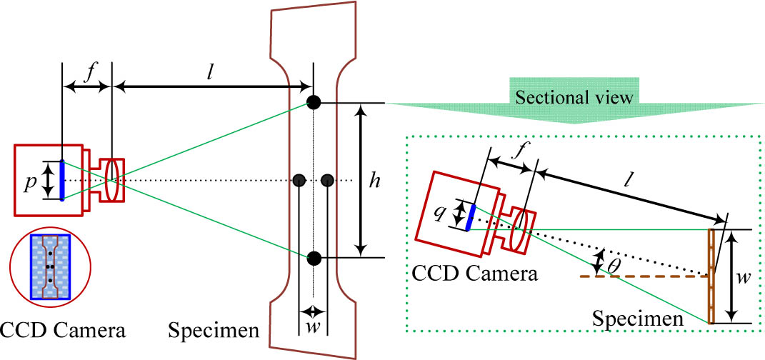
Plane calibration and coordinate calculation are essential in 2D vision measurement. The sub-pixel method is employed to determine the coordinates of specimen mark points or other geometric features in the calibration plane, and the coordinates can be calculated in the longitudinal and transverse directions simultaneously^[15]. According to the changes of the mark point coordinates and the pinhole model^[14], the measured geometric parameters can be calculated, such as the displacement, deformation, speed, etc. The view range is mainly determined by the focal length of the lens. By equipping lenses with different focal lengths, various view ranges can be obtained. The video extensometer is a typical application of 2D vision measurement for detecting the tensile deformation of materials, as shown in Fig. 1.

Figure 1.Video extensometer principle based on 2D vision measurement.

Usually, obvious round marks (although these are sometimes linear marks or random speckles) are made at both ends of the specimen. The marks project to the CCD; when the specimen is deformed, the imaging on the CCD changes accordingly. The real-time image data are input to the computer. The deformation can be calculated according to the imaging model through image processing and the location of the central coordinates. The conventional geometric similarity model is expressed as follows: $w \cos θ / q = h / p = l / f,$ (1)where $l$ and $f$ are measurement distance and lens focal length, $θ$ is the angle between the CCD image plane and the measurement plane, and $h$ , $w$ and $p$ , $q$ are the intervals measured and the image size, respectively.

Sign up for Chinese Optics Letters TOC. Get the latest issue of Chinese Optics Letters delivered right to you！Sign up now

The traditional 2D vision measurement method is based on the geometric similarity of the measurement plane and the image plane^[10,15]. The specimen surface is vertical to the optical axis and parallel to the image plane. According to the pinhole model^[14], the object and the image satisfy a similarity relation, and the actual geometric parameters of the specimen can be calculated by multiplying the parameters extracted from the image by the actual magnification. However, because of lens distortion and the difficulty of ensuring the verticality of the measurement plane and the optical axis^[16,17], the image and object planes are not strictly consistent with the pinhole model, which leads to low accuracy. In cases requiring high accuracy, the distorted image must first be corrected^[16,18], and then the image coordinates are extracted to calculate the actual parameters. But this method can only measure objects in the plane perpendicular to the optical axis, which is difficult to achieve in a practical operation, and a time-consuming calculation is required, which is not suitable for real-time measurements. The high-precision standard grid method requires specimens with specific surfaces to print the chessboard grid^[19]. When the specimen generates tension, mobility, or other changes, the grid is affected. According to the grid deformation information, the geometric parameters can be calculated^[20,21]. However, this requires a complicated operation, as each measurement demands that the specimen is printed with standard grids, and it cannot measure filaments and other small materials.

We propose a measurement approach based on local sub-plane mapping to establish a precise projection relationship between the image coordinates and real-world coordinates, which has the advantages of high robustness, the ability to measure a plane without a vertical axis, almost no restrictions regarding the specimen material, and no need for a distortion correction. A diagram of this method is shown in Fig. 2.

Figure 2.Process diagram of sub-planes: (a) calibration target with $6 \times 22$ point fixed to coincide with the specimen surface, (b) extract and save sub-pixel coordinates of every reference point from the target image, and (c) establish the mapping model between each image sub-plane and measurement plane.

As show in Fig. 2(a), a calibration target is needed to segment the sub-plane size and number accurately^[22]; it is fixed to coincide with the specimen’s surface in measurement plane. Then, the image is captured and processed to extract the sub-pixel coordinates of every reference point, as shown in Fig. 2(b). The grid array composed by these coordinates is saved in the computer for further locating. Thus, the image plane is divided into a series of sub-planes, and the mapping model is established between each image sub-plane and measurement plane, as shown in Fig. 2(c). The details of this mapping process are shown in Fig. 3.

Figure 3.Schematic of coordinate location method in sub-plane.

Thus, the image grids array can locate the measurement point according to the surrounding reference points extracted from the calibration plane. Figure 3 shows that the point $P^{'}$ on the specimen is found to be surrounded by $A^{'} B^{'} C^{'} D^{'}$ from the image grid array and $A B C D$ from the calibration target. In a small area, there exists an approximate affine invariance, as presented in ${\begin{cases} S_{Δ A P C} / S_{□ A B C D} = (S_{Δ A^{'} P^{'} C^{'}} / S_{□ A^{'} B^{'} C^{'} D^{'}}) / \cos θ \\ S_{Δ A P B} / S_{□ A B C D} = S_{Δ A^{'} P^{'} B^{'}} / S_{□ A^{'} B^{'} C^{'} D^{'}} \end{cases},$ (2)where $S_{Δ}$ and $S_{□}$ represent the areas of the triangle and the square, respectively, calculated by Heron’s formula. We obtain the standard distance from each axis: ${\begin{cases} d x = (2 d S_{Δ A^{'} P^{'} C^{'}} / S_{□ A^{'} B^{'} C^{'} D^{'}}) / \cos θ \\ d y = 2 d S_{Δ A^{'} P^{'} B^{'}} / S_{□ A^{'} B^{'} C^{'} D^{'}} \end{cases} .$ (3)

As long as the interval $d$ is known, the position of the tested point $P (x, y)$ can be determined. The normalized coordinates in the standard grid coordinates system are expressed in $P ((m + d x) d / \cos θ, (n + d y) d) .$ (4)

Assuming that the image coordinates of $A^{'} B^{'} C^{'} D^{'}$ and $P^{'}$ are $(x_{A^{'}}, y_{A^{'}})$ , $(x_{B^{'}}, y_{B^{'}})$ , $(x_{C^{'}}, y_{C^{'}})$ , $(x_{D^{'}}, y_{D^{'}})$ , and $(x^{'}, y^{'})$ , respectively, the transformation relationship between the image coordinates and practical geometric coordinates $P (x, y)$ is calculated using the following expression: ${\begin{matrix} x \approx d (m + \frac{2 \times | \det A_{A^{'} P^{'} C^{'}} |}{| \det A_{A^{'} B^{'} C^{'}} | + | \det A_{D^{'} B^{'} C^{'}} |}) / \cos θ \\ y \approx d (n + \frac{2 \times | \det A_{A^{'} P^{'} B^{'}} |}{| \det A_{A^{'} B^{'} C^{'}} | + | \det A_{D^{'} B^{'} C^{'}} |}) \end{matrix},$ (5)where $m$ and $n$ are the numbers of intervals on the chessboard from the origin, $d$ is the calibration target gauge length, $θ$ is the angle between the measurement plane and the image plane, as shown in Fig. 1, and $| det A |$ represents the absolute value of the area matrix $A$ determinant $| A |$ . This method avoids complex modeling. The impact of lens distortion can be suppressed. Its measurement accuracy and range largely depends on the calibration target accuracy and sub-planes area, respectively^[23,24].

As shown in Fig. 4, because of lens distortion, the measurement plane and image plane are not strictly consistent with the pinhole model^[16–18]. In order to demonstrate that the lens distortion effect is suppressed without loss of generality, we establish the image coordinate system with the origin as the center point of distortion. The undistorted coordinates of the four sub-plane vertexes surrounding point $P (x, y)$ are $A (x_{A}, y_{A})$ , $B (x_{A} + L, y_{A})$ , $C (x_{A}, y_{A} + L)$ , and $D (x_{A} + L, y_{A} + L)$ for a measurement angle of $θ = 0$ and a sub-plane side length $L$ . The distortion point $A^{'} (x_{A^{'}}, y_{A^{'}})$ and the corresponding point $A (x_{A}, y_{A})$ are related as follows: ${\begin{matrix} x_{A^{'}} = x_{A} R_{A} + [2 p_{1} x_{A} y_{A} + p_{2} (r_{A}^{2} + 2 x_{A}^{2})] \\ y_{A^{'}} = y_{A} R_{A} + [2 p_{2} x_{A} y_{A} + p_{1} (r_{A}^{2} + 2 y_{A}^{2})] \end{matrix},$ (6)where $R_{A} = 1 + k_{1} r_{A}^{2} + k_{2} r_{A}^{4} + k_{3} r_{A}^{6}$ , and $r_{A} = {[x_{A}^{2} + y_{A}^{2}]}^{1 / 2}$ , $k_{1}$ , $k_{2}$ , and $k_{3}$ are the coefficients of the radial distortion, and $p_{1}$ and $p_{2}$ are the coefficients of the tangential distortion^[25]. The other points also satisfy this distortion relationship. Thus, the areas of $S_{Δ}$ and $S_{□}$ shown in Fig. 4 can be calculated using the coordinates of $A B C D$ , $A^{'} B^{'} C^{'} D^{'}$ , $P$ , and $P^{'}$ . The real transverse and longitudinal deviation of $P (x, y)$ and $P^{'} (x^{'}, y^{'})$ are then given by the following expressions: ${\begin{matrix} Δ x = x^{'} - x = (2 \frac{S_{Δ A^{'} P^{'} C^{'}}}{S_{□ A^{'} B^{'} C^{'} D^{'}}} - \frac{x - x_{A}}{x_{B} - x_{A}}) d \\ Δ y = y^{'} - y = (2 \frac{S_{Δ A^{'} P^{'} B^{'}}}{S_{□ A^{'} B^{'} C^{'} D^{'}}} - \frac{y - y_{A}}{y_{C} - y_{A}}) d \end{matrix} .$ (7)

Figure 4.Effects of the lens distortion: (a) real chessboard image and image with lens distortion and (b) pixel deviations before and after image distortion.

It is reasonable to adopt this analysis to assess the performance of the measurement method rather than that of the feature-extraction algorithm, which is used to localize the distorted image points. We know the distortion coefficient of the lens and know that the measurement view range is $400 mm \times 400 mm$ , which is larger than that for the real measurement. The computer-simulated deviation data between the undistorted and measured coordinates are presented in Fig. 5.

Figure 5.Relationship between sub-planes interval and mapping accuracy, obtained using lens with first distortion coefficient $k_{1} = 4.1 \times 10^{- 8}$ : (a) fixed interval deviation distribution in whole view range $400 mm \times 400 mm$ and (b) relationship between maximum deviation and sub-planes interval.

Figure 5(a) displays the deviation distribution over the entire view range when the sub-plane interval was fixed as 6 mm (equal to the calibration target gauge length in the real experiment). We see that the maximum deviation obtained by the local sub-plane mapping of the 2D vision measurement was 2.4 μm when the view range was $400 mm \times 400 mm$ . Figure 5(b) shows the relationship between the maximum deviation value and the sub-plane interval in the same view range. Thus, when designing calibration target, an appropriate gauge length can be chosen according to the accuracy requirements.

In the measurement process, the three fundamental planes are the calibration plane, the measurement plane, and the image plane. The specimen is loaded almost coincident with the calibration plane, in accordance with the mechanical constraints to reduce the out-plane effects. But since the out-plane effects still exist, it is necessary to analyze the out-plane deviation, as shown in Fig. 6.

Figure 6.Principle of the out-plane effects.

According to the pinhole model, the relationship between the measurement plane and the image plane can be expressed by the following equation: $d / f = h / l,$ (8)where $d$ and $f$ are the measurement distance and the lens focal length, respectively. $h$ is the distance measured, and $l$ is the size of the imaging distance. Thus, the deviation $Δ h$ caused by the out-plane displacement $Δ d$ can be expressed as $Δ h = h^{'} - h = (l^{'} \times Δ d) / f,$ (9)where $h^{'}$ and $l^{'}$ are the actual measurement distance and image size, respectively. The relative measurement accuracy can be expressed by the following equation: $δ = Δ h / h^{'} = Δ d / (d - Δ d) .$ (10)

In actual applications, the relative accuracy of 2D vision measurement usually is no more than 5%, which can be satisfied by designing the appropriate measurement distance and the precision of the mechanical constraints and compensating for the specimen’s thickness.

The proposed method was tested in real experiments and compared with conventional 2D vision measurement methods, including the geometric similarity method and digital image correlation (DIC). As a classic microscopic measurement method for in-plane displacement and deformation, the DIC has an important application in 2D vision measurement^[26]. Though the local sub-plane mapping method has a large measurement range and the DIC method is too time-consuming to suit that, the comparison between the two methods was performed over an approximately 1 mm range. In the experiments, the calibration target was a chessboard pattern with $6 \times 22$ circular points distributed evenly, where the distance between the adjacent points was 6 mm. The lens was a PenTax H1214-M made in Japan, with a horizontal view angle of 28.91° and a 12 mm focal length, and a PointGrey Flea3 camera made in Canada with 1/2.8” CCD was used. The image resolution was 1920 pixels × 2416 pixels, whose 1/3 part of 640 pixels × 2416 pixels was used for the experiments. The measurement distance was 45 cm and the accuracy of sub-pixel location usually could achieve 0.02 pixels^[27]. Thus, the accuracy of the sub-pixel location was 1.25 μm. The circular mark was approximately 6 mm in diameter, and the size of the DIC subset was 81 pixels × 81 pixels. The images for calibration and measurement were captured from a random orientation, and the position of the CCD camera was fixed throughout.

First, the plane calibration was performed using two images of the calibration target. One image of the calibration target was captured and stored. The coordinates array of the reference grids could be extracted through image processing methods such as image filtering, edge detection, and feature extraction. Then, another image was captured and processed according the former process, whose grid coordinates could be normalized according to the reference grid array by Eq. (4). Thus, the intervals of the adjacent points of the second image were calculated, and the calibration accuracy was expressed by the average, minimum, and maximum errors between the actual intervals and the gauge length of the calibration target. In the measurement process, a series of images of the specimen with circular marks were captured and processed in real time. If the marks were in the calibrated area, the real-time normalized coordinates of the specimen marks could be calculated and the position of each mark was located. The entire measurement process is shown in Fig. 7.

Figure 7.Process of measurement experiment: (a) calibration target fixed on stretching machine, (b) image for calibration, (c) matrix of circular center, (d) displacement measurement using two methods, (e) 81 pixels × 81 pixels correlation subset, and (f) gauge length measurement.

To practically determine the measurement accuracy, we performed two comparison tests. The first was round-mark point-displacement test. It used a high-precision stretching machine to load the displacement, and the measurement data was compared with the results measured by the DIC method and the displacement data from the stretching machine. The second was a gauge length measurement experiment, where the interval between two adjacent round mark points was known, and the measurement data of the distance was compared with the standard length data.

The calibration results obtained using different methods are compared in Fig. 8 and Table 1. The measurement results are compared in Tables 2 and 3. Clearly, the calibration methods greatly influence the measurement accuracy, and the local sub-plane mapping method has better accuracy and stability. Tables 2 and 3 present comparative results for the real-time measurement of the random displacement and gauge length. The real data for the random displacement were captured by the stretching machine, and that for the gauge length were obtained using the calibration target. Two kinds of contrast indicate that the accuracy of this mapping method is better than an absolute accuracy of 3 μm in a small measurement range, and a relative accuracy of 1% in a large measurement range, which is better than that of the conventional geometric similarity method and is comparable to the DIC method.

Figure 8.Comparative results for calibration accuracy using the two methods.

Calibration Accuracy		Number	Maximum (μm)	Minimum (μm)	Average (μm)	Maximum (%)	Minimum (%)
Local Sub-Plane	X	136	1.94	0.00	1.00	0.32	0.00
Mapping Method	Y	136	2.16	0.00	1.00	0.36	0.00
Geometric Similarity	X	136	28.08	0.12	12.22	4.68	0.02
Method	Y	136	27.62	0.15	13.07	4.60	0.03

Table 1. Comparison of Calibration Accuracy

View all Tables

Displacement Measurement/μm	Data Comparison
Proposed Method	103	217	354	496	615	749	905	1103
DIC Method	102	217	359	501	616	750	909	1104
Real Data	103.7	218.2	356.1	497.8	614.3	747.7	907.1	1101.5

Table 2. Comparison of Displacement Measurement Accuracy

View all Tables

Gauge Length Measurement/μm	Data Comparison
Proposed Method	5998	11995	18008	24014	35991	59,984	84,017
Real Data	6000	12000	18000	24000	36000	60,000	84,000

Table 3. Comparison of Gauge Length Measurement Accuracy

View all Tables

In conclusion, we propose a precise measurement approach for 2D vision measurement. Until now, the conventional geometric similarity methods based on whole-plane mapping have led to decreased accuracy because of lens distortion. Moreover, the condition that the measured object surface is vertical to the optical axis of the camera system and parallel to the image plane is unrealistic. To overcome these shortcomings, the local sub-plane mapping method is presented for the first time, with the aim of establishing a precise transformation between the image point and the real-world point in a 2D plane. Additionally, the local sub-plane mapping model and simple algorithm for coordinate location are combined to improve the measurement accuracy and efficiency. To validate the performance of the proposed method, we performed experiments using synthetic and real data and compared the results with those for the conventional method. The results from the computer simulation and real data demonstrate the advantage of the proposed approach.

References

[1] S. Shirmohammadi, A. Ferrero. IEEE Instru. Meas. Mag., 17, 41(2014).

[2] F. Zhou, Y. Wang, B. Peng, Y. Cui. Meas. J. Int. Meas. Confed., 46, 1147(2013).

[3] Z. Y. Zhang. IEEE Trans. Pattern Anal. Mach. Intell., 22, 1330(2000).

[4] Z. Ren, J. Liao, L. Cai. Appl. Opt., 49, 1789(2010).

[5] R. Jachyma, K. Kwiecińskia. Weld. Int., 28, 39(2014).

[6] Y. Yin, D. Xu, Z. Zhang, X. Wang, W. Qu. J. Elec. Meas. Instrum., 27, 347(2013).

[7] F. Zhou, E. Zappa, L. C. Chen. Adv. Mech. Eng., 947610(2014).

[8] B. Wu, Y. Zhang. Adv. Mech. Eng., 5, 587904(2013).

[9] H. Jiang, H. Zhao, X. Li. Opt. Lasers Eng., 50, 1484(2012).

[10] L. Xu, X. Li, X. Lv. Mech. Eng. Autom., 1, 73(2006).

[11] W. Zhang, H. Bai. Phys. Test. Chem. Anal., 48, 174(2012).