
Shixin Ma, Chuntong Liu, Hongcai Li, Geng Zhang, Zhenxin He. Feature Extraction Based on Linear Embedding and Tensor Manifold for Hyperspectral Image[J]. Acta Optica Sinica, 2019, 39(4): 0412001
- Acta Optica Sinica
- Vol. 39, Issue 4, 0412001 (2019)
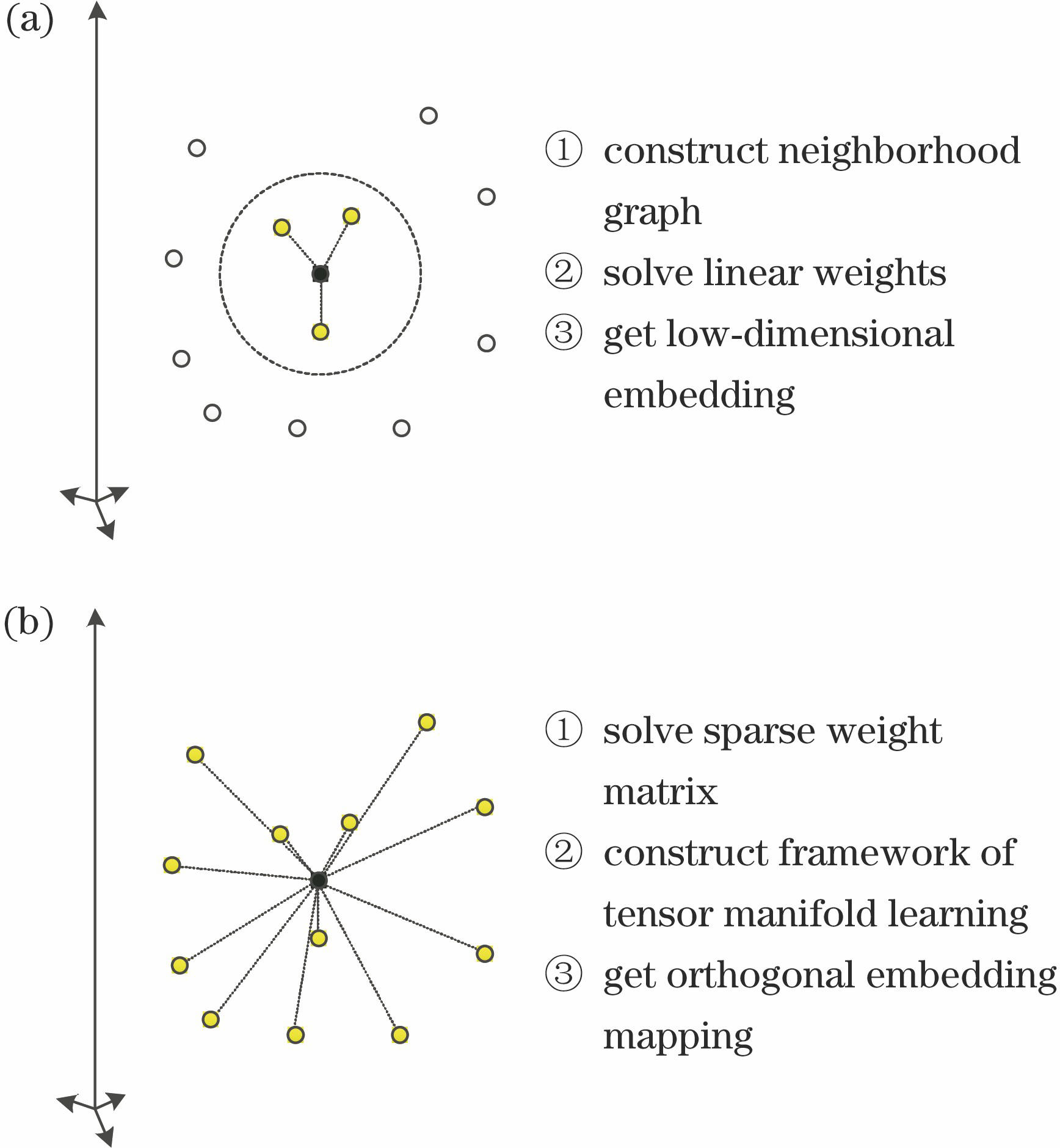
Fig. 1. Diagrams of manifold difference. (a) LLE algorithm; (b) GLE algorithm
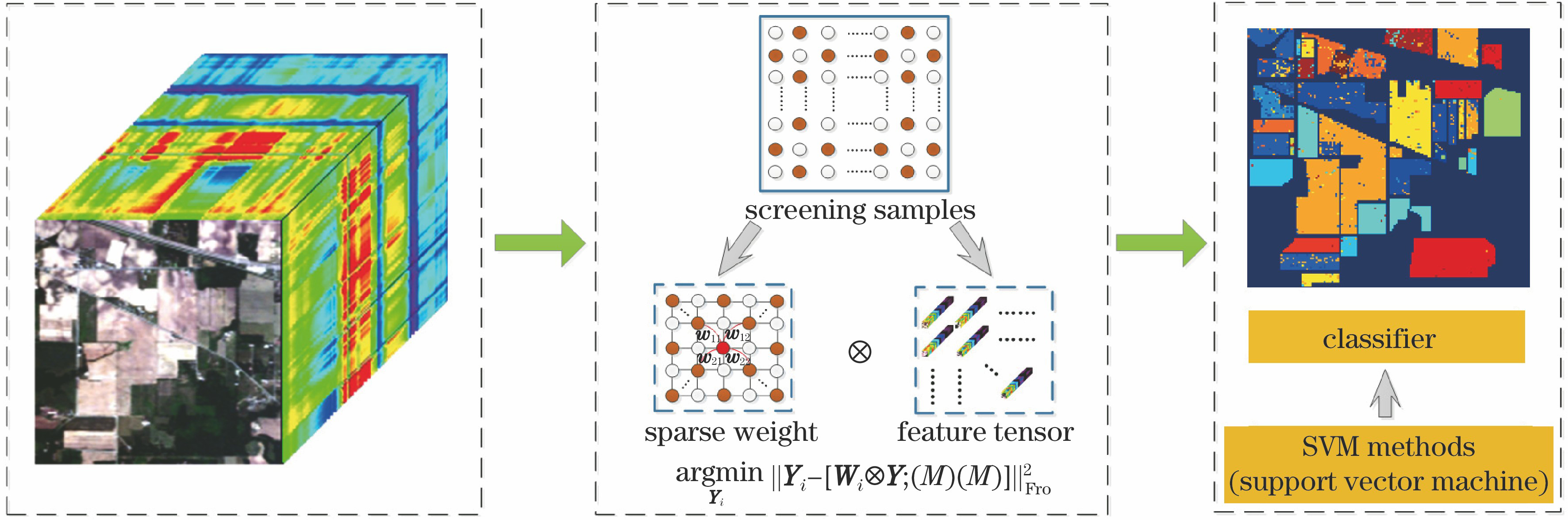
Fig. 2. Dimensionality reduction frame of tensor manifold
Fig. 3. Indian Pines hyperspectral data. (a) Pseudo-color image; (b) ground-truth map
Fig. 4. PaviaU hyperspectral data. (a) Pseudo-color image; (b) ground-truth map
Fig. 5. Influence of sparse parameters λ on classification performance (Indian Pines data)
Fig. 6. Dimensionality reduction performance of Indian Pines data obtained with different algorithms. (a) Ground-truth map; (b) PCA algorithm; (c) MNF algorithm; (d) LLE algorithm; (e) LE algorithm; (f) LPP algorithm; (g) RP algorithm; (h) proposed algorithm
Fig. 7. Dimensionality reduction performance of PaviaU data obtained with different algorithms. (a) Ground-truth map; (b) PCA algorithm; (c) MNF algorithm; (d) LLE algorithm; (e) LE algorithm; (f) LPP algorithm; (g) RP algorithm; (h) proposed algorithm
Fig. 8. Projection results obtained with different dimensionality reduction algorithms (Indian Pines data). (a) Original data (band 1 & 2); (b) PCA algorithm; (c) MNF algorithm; (d) LLE algorithm; (e) LE algorithm; (f) LPP algorithm; (g) RP algorithm; (h) proposed algorithm
Fig. 9. Classification accuracy of different algorithms obtained at different embedding dimensions. (a) Indian Pines data; (b) PaviaU data
|
Table 1. Classification accuracy of different dimensionality reduction algorithms
|
Table 2. Time complexity of different algorithms
| ||||||||||||||||||||||||||||||||||||||||||||||||||||||||||||||||||
Table 3. Computation time of different algorithms

Set citation alerts for the article
Please enter your email address
© Copyright 2018-2021 | Chinese Laser Press. All Rights Reserved 沪ICP备15018463号-20