Hyperspectral Image Classification Combined Dynamic Convolution with Triplet Attention Mechanism

Aili Wang; Meihong Liu; Dong Xue; Haibin Wu; Lanfei Zhao; Iwahori Yuji

doi:10.3788/LOP202259.1015011

Journals >Laser & Optoelectronics Progress >Volume 59 >Issue 10 >Page 1015011 > Article

Laser & Optoelectronics Progress
Vol. 59, Issue 10, 1015011 (2022)

Hyperspectral Image Classification Combined Dynamic Convolution with Triplet Attention Mechanism

Aili Wang¹, Meihong Liu¹, Dong Xue¹, Haibin Wu^1、*, Lanfei Zhao¹, and Iwahori Yuji²

Author Affiliations

¹Heilongjiang Province Key Laboratory of Laser Spectroscopy Technology and Application, College of measurement and control technology and communication Engineering, Harbin University of Science and Technology, Harbin 150080, Heilongjiang , China

²Department of Computer Science, Chubu University, Aichi 487-8501, Japan

show less

DOI: 10.3788/LOP202259.1015011 Cite this Article Set citation alerts

Aili Wang, Meihong Liu, Dong Xue, Haibin Wu, Lanfei Zhao, Iwahori Yuji. Hyperspectral Image Classification Combined Dynamic Convolution with Triplet Attention Mechanism[J]. Laser & Optoelectronics Progress, 2022, 59(10): 1015011 Copy Citation Text

show less

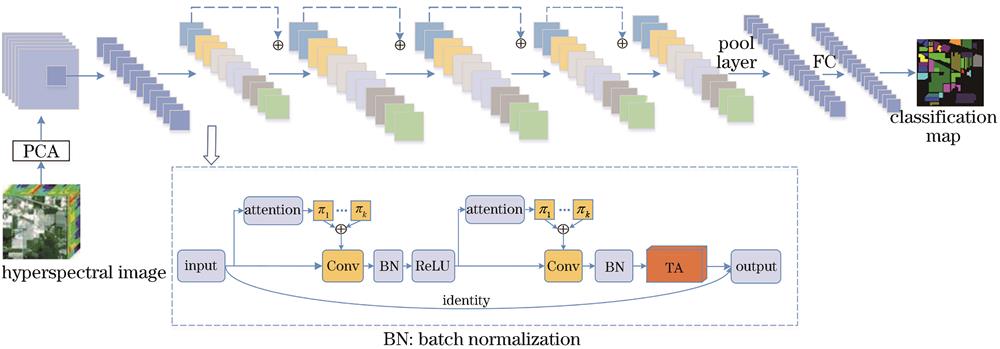
Fig. 1. Flow chart of hyperspectral image classification algorithm combined dynamic convolution with triple attention mechanism

Download full size

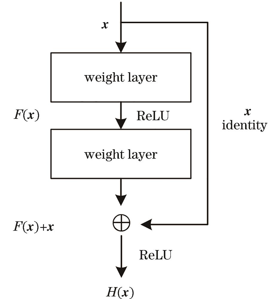
Fig. 2. Residual unit structure diagram of ResNet

Download full size

Fig. 3. Dynamic perceptron

Download full size

Fig. 4. Dynamic convolution

Download full size

Fig. 5. TA schematic diagram

Download full size

Fig. 6. Architecture diagram of TA

Download full size

Fig. 7. False color map and ground truth map of each dataset. (a) Pavia University; (b) Kennedy Space Center; (c) Salinas

Download full size

Fig. 8. Comparative analysis of overall classification accuracy of different classification algorithms

Download full size

Fig. 9. Classification results of Pavia University dataset. (a) Ground truth; (b) RBF-SVM; (c) EMP-SVM; (d) DCNN; (e) GAN; (f) ResNet; (g) PyResNet; (h) DTAResNet

Download full size

Fig. 10. Classification results of Kennedy Space Center dataset. (a) Ground truth; (b) RBF-SVM; (c) EMP-SVM; (d) DCNN; (e) GAN; (f) ResNet; (g) PyResNet; (h) DTAResNet

Download full size

Fig. 11. Classification results of Salinas dataset. (a) Ground truth; (b) RBF-SVM; (c) EMP-SVM; (d) DCNN; (e) GAN; (f) ResNet; (g) PyResNet; (h) DTAResNet

Download full size

Parameter	Dataset
Parameter	Pavia University	Kennedy Space Center	Salinas
Sensor	ROSIS	AVIRIS	AVIRIS
Size /（pixel×pixel）	610×340	512×614	512×217
Resolution /m	1.3	18	3.7
Spectral band	103	176	204
Land-cover	9	13	16
Total sample pixel	42776	5211	54129

Table 1. Experimental dataset parameters

Layer name	Output size	ResNet-34 parameter setting
Conv1	$5 \times 5$	$7 \times 7$ ，64，stride 2
Conv2_x	$3 \times 3$	$3 \times 3$ max pool，stride 2
Conv2_x	$3 \times 3$	$[\begin{array}{l} 3 \times 3,64 \\ 3 \times 3,64 \end{array}] \times 3$
Conv3_x	$2 \times 2$	$[\begin{array}{l} 3 \times 3,128 \\ 3 \times 3,128 \end{array}] \times 4$
Conv4_x	$1 \times 1$	$[\begin{array}{l} 3 \times 3,256 \\ 3 \times 3,256 \end{array}] \times 6$
Conv5_x	$1 \times 1$	$[\begin{array}{l} 3 \times 3,512 \\ 3 \times 3,512 \end{array}] \times 3$

Table 2. Parameter settings of ResNet-34

Class	RBF-SVM	EMP-SVM	DCNN	GAN	ResNet	PyResNet	DTAResNet
Asphalt	88.51±2.44	89.06±1.33	90.59±0.62	94.97±2.09	95.59±3.43	95.55±0.25	96.35±0.64
Meadows	88.86±3.52	88.12±0.23	89.26±1.05	97.62±1.96	97.10±2.06	98.91±0.71	99.16±0.32
Gravel	78.51±2.93	78.65±3.05	78.89±2.65	89.53±3.62	87.53±5.27	93.81±4.60	91.09±1.07
Trees	86.17±1.28	88.95±0.53	89.05±1.45	96.72±0.85	99.03±0.33	99.35±0.28	99.57±0.18
Metal	94.11±2.36	93.23±1.29	94.55±0.67	97.94±0.99	98.56±1.36	99.67±0.17	99.81±0.13
Bare Soil	90.11±0.62	90.13±0.54	90.23±1.23	96.34±1.43	98.35±1.06	98.39±0.18	99.05±0.62
Bitumen	82.13±2.52	81.66±3.31	83.69±2.82	98.73±1.12	99.29±0.51	92.31±0.88	99.41±0.39
Bricks	82.38±2.57	83.05±1.61	83.57±2.91	95.01±1.05	94.61±0.50	89.44±4.66	89.96±3.07
Shadows	93.29±0.55	95.26±0.56	94.68±0.46	97.39±0.97	99.39±0.58	98.96±0.56	98.42±1.45
OA /%	90.65±1.32	91.07±0.85	91.32±1.22	93.88±2.28	96.49±1.78	97.05±0.45	97.49±0.24
AA /%	87.11±2.09	87.57±1.38	88.28±1.54	95.82±1.56	96.61±1.68	96.27±1.36	96.98±1.57
100K	88.92±1.46	88.72±1.44	89.43±1.09	92.93±1.94	95.31±2.41	96.22±0.11	96.67±0.32

Table 3. Classification results of Pavia University dataset

Class	RBF-SVM	EMP-SVM	DCNN	GAN	ResNet	PyResNet	DTAResNet
Scrub	92.11±2.32	93.42±1.38	92.48±2.21	95.29±0.45	96.00±1.75	96.24±0.43	96.63±2.65
Willow	82.25±1.52	83.66±2.65	83.96±2.82	80.83±2.42	92.82±2.80	93.24±0.54	97.68±0.49
Palm	85.37±3.64	85.69±3.21	73.52±4.98	89.43±1.96	88.67±2.91	87.62±1.72	89.98±0.76
Pine	60.08±4.33	62.43±5.63	60.22±8.52	83.02±2.43	76.80±3.46	86.01±1.91	86.02±0.64
Broadleaf	62.56±5.98	64.42±4.65	61.09±5.90	96.15±1.53	78.50±1.63	77.55±2.67	76.15±1.53
Hardwood	65.38±3.45	67.65±5.10	64.24±5.24	95.82±1.91	79.43±2.93	86.15±1.24	96.80±0.30
Swap	63.52±5.66	65.56±6.36	65.95±7.24	95.16±0.85	75.88±2.90	84.70±1.68	82.68±1.85
Graminoid	71.52±3.84	73.28±2.98	73.60±3.22	75.78±2.10	96.10±1.75	96.17±0.39	96.52±0.13
Spartina	81.56±4.55	85.32±3.55	86.94±2.84	95.23±2.24	93.93±3.30	94.28±0.54	96.82±2.24
Cattail	90.78±1.84	93.25±1.22	93.52±0.98	98.98±0.38	96.77±1.34	99.30±0.05	99.48±0.38
Salt	93.65±1.46	95.38±2.01	95.91±0.55	96.06±0.93	99.51±0.48	99.54±0.06	99.98±0.01
Mud	90.35±2.19	91.01±2.58	89.39±1.20	96.37±1.32	97.09±0.95	96.30±0.47	92.44±1.91
Water	99.26±0.24	99.31±0.32	99.84±0.04	99.09±0.14	99.65±0.05	99.28±0.18	99.85±0.33
OA /%	80.65±3.08	81.97±3.27	81.04±2.90	93.56±0.98	89.93±2.54	94.01±1.08	94.93±1.83
AA /%	79.87±3.16	81.57±3.20	80.05±3.52	92.09±1.44	90.11±2.02	92.03±0.91	93.16±1.00
100K	79.93±3.45	80.78±2.96	79.67±3.78	92.85±1.56	88.86±4.96	93.16±2.04	94.35±1.98

Table 4. Classification results of Kennedy Space Center dataset

Class	RBF-SVM	EMP-SVM	DCNN	GAN	ResNet	PyResNet	DTAResNet
Brocoli_green_weeds_1	83.42±1.56	96.16±0.28	97.75±0.22	85.71±1.23	99.25±0.05	99.90±0.06	99.95±0.02
Brocoli_green_weeds_2	92.19±0.85	99.27±0.02	97.19±0.14	87.50±1.05	99.35±0.20	99.95±0.03	99.99±0.01
Fallow	90.66±1.94	80.45±1.78	78.39±0.12	80.46±2.13	99.35±0.48	99.03±0.03	99.97±0.02
Fallow_rough_plow	95.33±1.92	98.34±0.35	99.07±0.08	99.90±0.01	97.49±1.80	99.24±0.05	98.93±1.38
Fallow_smooth	86.52±2.64	94.56±1.32	98.84±0.23	90.35±1.06	99.32±0.43	99.61±0.01	99.71±0.23
Stubble	97.62±0.25	99.45±0.09	99.86±0.55	99.34±0.33	99.46±0.02	99.76±0.06	99.98±0.01
Celery	95.22±0.74	97.36±0.65	99.09±0.29	99.90±0.03	99.38±0.01	99.96±0.01	99.99±0.01
Grapes_untrained	84.35±2.61	84.38±0.46	94.96±1.23	90.95±1.08	96.39±0.47	95.45±1.28	96.61±1.23
Soil_vinyard_develop	98.45±0.45	98.74±1.06	99.69±0.02	99.92±0.03	99.47±0.02	99.88±0.02	99.97±0.02
Corn_senesced_green_weeds	80.55±4.69	91.98±0.91	99.25±0.15	98.23±0.65	99.70±0.05	99.83±0.01	99.72±0.15
Lettuce_romaine_4wk	85.55±3.13	90.73±3.22	92.19±1.68	97.56±0.84	98.71±1.25	99.15±0.09	99.23±1.08
Lettuce_romaine_5wk	96.04±0.69	99.79±0.10	99.89±0.19	99.04±0.42	99.52±0.24	99.80±0.01	99.90±0.07
Lettuce_romaine_6wk	98.54±0.43	98.22±0.65	94.78±2.09	80.62±2.56	99.68±0.15	99.06±0.32	99.63±0.29
Lettuce_romaine_7wk	86.33±1.88	96.23±0.24	95.85±0.67	80.21±2.91	99.45±0.54	99.70±0.24	99.33±0.37
Vinyard_untrained	66.78±6.66	63.89±6.32	93.85±1.89	79.99±0.59	94.04±1.52	94.79±2.17	95.58±1.89
Vinyard_vertical_trellis	83.72±4.84	79.78±5.12	99.95±0.02	91.08±0.72	99.20±0.68	98.68±0.33	99.92±0.02
OA /%	87.79±2.65	89.74±1.43	96.38±0.76	95.00±1.45	98.25±0.28	98.18±0.38	98.65±0.13
AA /%	88.83±2.21	91.83±1.41	96.29±0.60	91.30±0.98	98.73±0.48	98.99±0.29	99.30±0.40
100K	88.93±1.97	88.96±2.05	95.66±0.93	93.31±1.36	98.05±0.31	97.97±0.04	98.17±0.23