
Luoru Li, Xin Xu, Hao Dong, Rong Gui, Xinfang Xie. Gaussian Mixture Model and Classification of Polarimetric Features for SAR Images[J]. Acta Optica Sinica, 2019, 39(1): 0128002
- Acta Optica Sinica
- Vol. 39, Issue 1, 0128002 (2019)
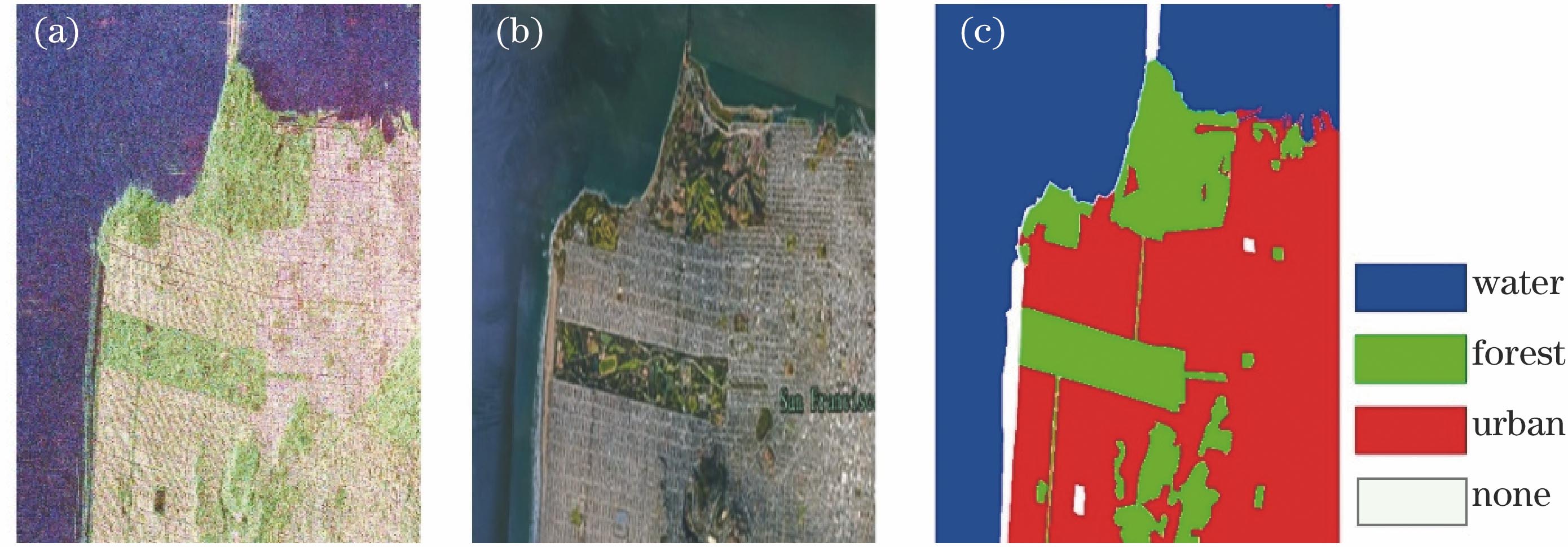
Fig. 1. Polarimetric SAR images from Radarsat-2 in San Francisco. (a) Pauli pseudo color image; (b) corresponding map; (c) ground truth
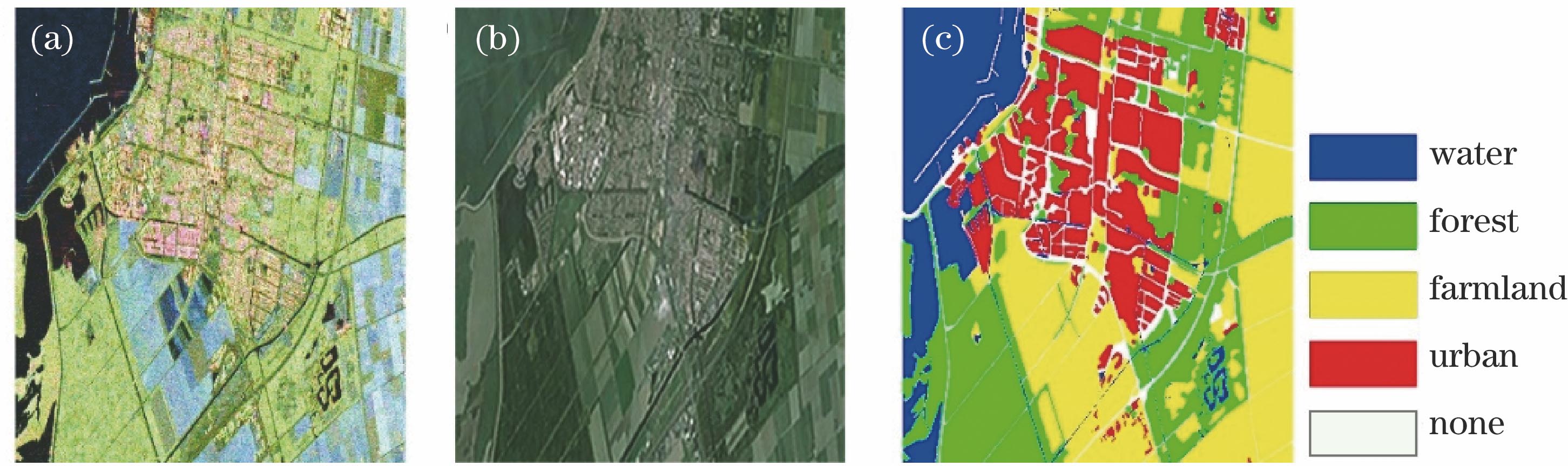
Fig. 2. Polarimetric SAR images from Radarsat-2 in Flevoland. (a) Pauli pseudo color image; (b) corresponding map; (c) ground truth
Fig. 3. Polarimetric SAR images from Radarsat-2 in Vancouver. (a) Pauli pseudo color image; (b) corresponding map; (c) ground truth
Fig. 4. Fitting results of each feature at different distributions. (a) Water; (b) forest; (c) farmland; (d) urban
Fig. 5. Flow chart of constrained distance estimation algorithm
Fig. 6. Distance function at different parameters
Fig. 7. Fitting results at different parameters. (a) k=1; (b) k=5; (c) k=8
Fig. 8. Flow chart of polarimetric SAR image classification algorithm based on GMM model
Fig. 9. Polarimetric SAR classification results in San Francisco. (a) KNN; (b) SVM; (c) RF; (d) WHRT; (e) GMM
Fig. 10. Polarimetric SAR classification results in Flevoland. (a) KNN; (b) SVM; (c) RF; (d) WHRT; (e) GMM
Fig. 11. Polarimetric SAR classification results in Vancouver. (a) KNN; (b) SVM; (c) RF; (d) WHRT; (e) GMM
Fig. 12. Overall accuracy vs. number of training samples
|
Table 1. KS distance mean at different distributions
|
Table 2. Maximum KS distance at different distributions
|
Table 3. Experimental accuracy in classification of polarimetric SAR%
|
Table 4. Experimental accuracy in classification of polarimetric SAR under different features in Flevoland%

Set citation alerts for the article
Please enter your email address
© Copyright 2018-2021 | Chinese Laser Press. All Rights Reserved 沪ICP备15018463号-20