Fig. 1. Illustration of multifunctional OMs and the material optical properties. (a) Scheme of structured Sb2Te3 OMs for optical data encryption. (b) Structure design and related parameters of meta-unit. The periods Px and Py of meta-cell are 300 nm. The MIM layers’ thicknesses h1, h2, and h3 are 30, 90, and 130 nm, respectively. (c) Distribution of the propagation phase with the size of meta-unit. (d) Distribution of PB phases with the rotation angle of meta-unit. (e), (f) Refractive index n and extinction coefficient k of Sb2Te3 in (e) amorphous and (f) crystalline states [58].

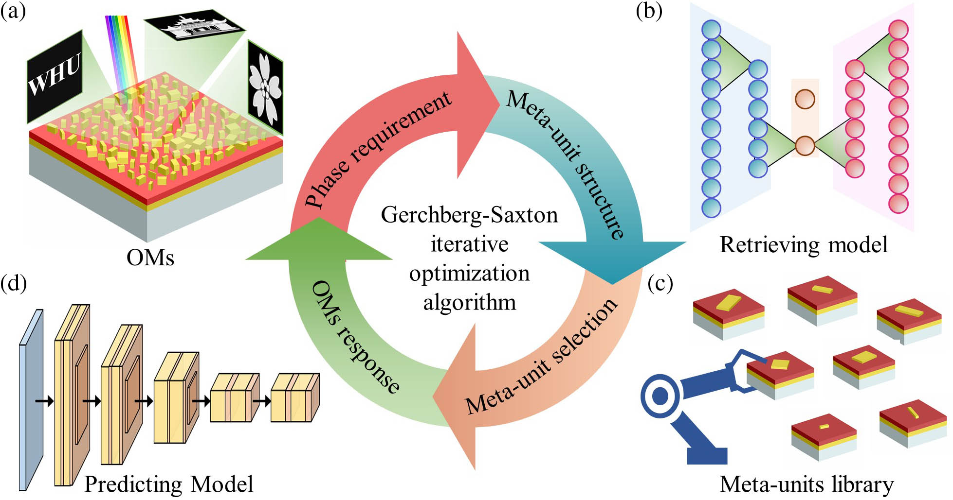
Fig. 2. Design process for the multifunctional OMs. (a) Proposed multifunctional OMs, (b) retrieving network model, (c) meta-unit library, and (d) predicting network model. These two deep learning network models are integrated into the GS iterative optimization algorithm, enabling bidirectional linkage between design objectives and OM geometric parameters.

Fig. 3. Schematic diagram of the deep learning model for a single meta-unit design. (a) The design parameters of the meta-unit and the crystalline phase organization of Sb2Te3 are amorphous. (b) Predicting model for reflectance spectra and (c) retrieving model of the required intensity and phase. The forward prediction from design parameters to reflection spectra is fixed, whereas the on-demand inverse design process is characterized by uncertainty, thus ensuring the multiplicity of design outcomes.

Fig. 4. Training results of the forward predicting network model. (a) Datasets for the forward deep learning network. The total data quantity of each cuboid is 23,328. (b) Distribution of datasets. (c) Correlation analysis of parameters. (d) Training and validation loss of X polarization, LCP, and RCP at wavelength of 520 nm.

Fig. 5. Training results of the retrieving model. (a) Distribution of datasets and (b) correspondence among the real, predicted, and generated values of X polarization, LCP, and RCP. The black plot represents the target values, the red plot represents the predicted values, and the blue plot represents the generated values. (c) Pearson correlations among the real, predicted, and generated values for each polarization.

Fig. 6. Intensity and phase regeneration results of the retrieving model. Comparison images among the target phase, target image, reconstructed phase, and reconstructed image for each polarization state.

Fig. 7. Target image and calculated results of multifunctional OMs under X polarization, LCP, and RCP. These calculated results are obtained through the combination of simulation results and the utilization of Fraunhofer diffraction integrals.

Table 1. Detailed Configuration of the Predicting Model

Table 2. Detailed Configuration of the Retrieving Model