
Daisy Williams, Xiaoyi Bao, and Liang Chen, "Characterization of high nonlinearity in Brillouin amplification in optical fibers with applications in fiber sensing and photonic logic," Photonics Res. 2, 1 (2014)
- Photonics Research
- Vol. 2, Issue 1, 1 (2014)
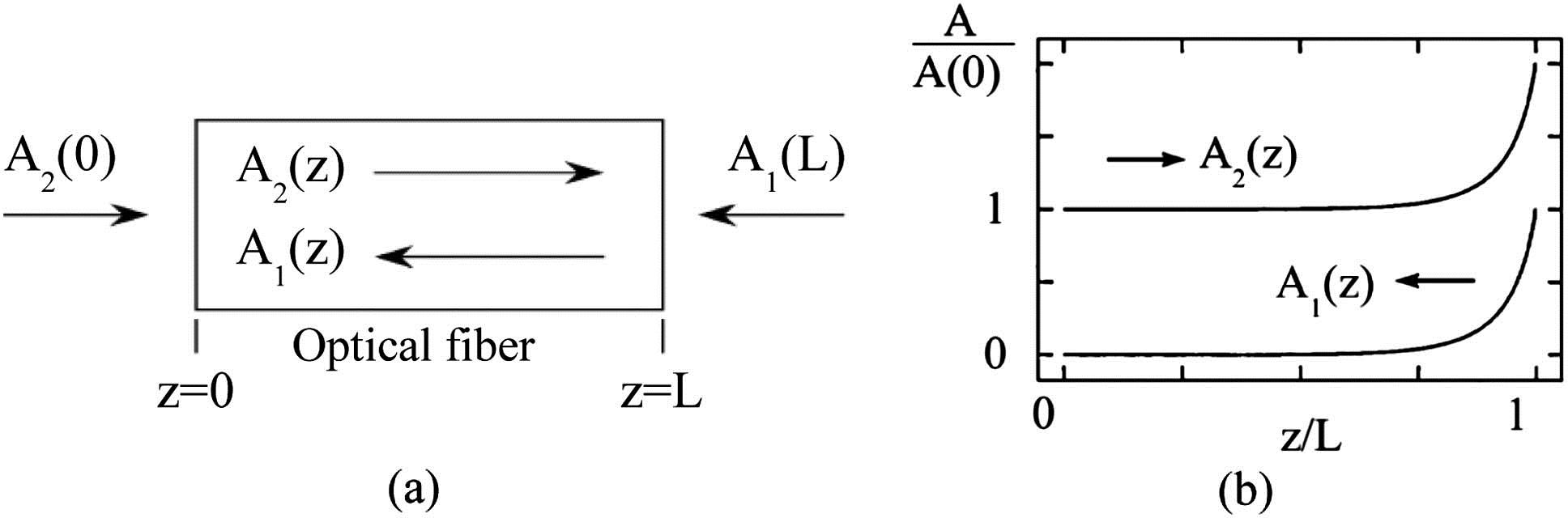
Fig. 1. (a) Schematic arrangement of SBS in a fiber of length L A 1 ( z ) A 2 ( z )
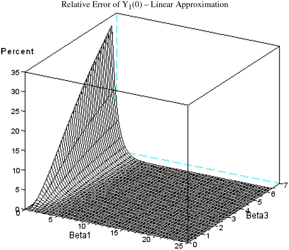
Fig. 2. Relative error of linear approximation of 3D parametric model of output CW. L = 1000 m 0 < P pump < 10 mW 0 < P probe < 40 mW
Fig. 3. Relative error of quadratic approximation of 3D parametric model of output CW. L = 1000 m 0 < P pump < 10 mW 0 < P probe < 40 mW
Fig. 4. Linear approximation of 3D parametric model of output CW. Dimensionless output intensity of the CW versus dimensionless parameters β 1 β 3 γ e = 0.902 v = 5616 m / s n = 1.48 λ = 1.319 μm ρ 0 = 2.21 g / cm 3 Γ B = 0.1 GHz L = 1000 m 0 < P pump < 10 mW 0 < P probe < 40 mW
Fig. 5. Linear approximation of 3D parametric model of output PW. Dimensionless output intensity of the PW versus dimensionless parameters β 1 β 3 γ e = 0.902 v = 5616 m / s n = 1.48 λ = 1.319 μm ρ 0 = 2.21 g / cm 3 Γ B = 0.1 GHz L = 1000 m 0 < P pump < 10 mW 0 < P probe < 40 mW
Fig. 6. Analytical results, normalized intensity units. P PW n = 1.48 γ e = 0.902 λ = 1319 nm ρ 0 = 2.21 g / cm 3 v = 5616 m / s L = 1000 m Γ B = 0.1 GHz P CW = 1.0 mW
Fig. 7. Pump depletion as a function of probe spectral distortion. P PW n = 1.48 γ e = 0.902 λ = 1319 nm ρ 0 = 2.21 g / cm 3 v = 5616 m / s L = 1000 m Γ B = 0.1 GHz P CW = 1.0 mW
Fig. 8. Shaded area depicts range of β 1 β 3
Fig. 9. Experimental setup.
Fig. 10. Experimental results, normalized intensity units. P PW n = 1.48 γ e = 0.902 λ = 1319 nm ρ 0 = 2.21 g / cm 3 v = 5616 m / s L = 1000 m Γ B = 0.1 GHz P CW = 1.0 mW


Set citation alerts for the article
Please enter your email address

© Copyright 2018-2021 | Chinese Laser Press. All Rights Reserved 沪ICP备15018463号-20