Daisy Williams, Xiaoyi Bao, and Liang Chen, "Characterization of high nonlinearity in Brillouin amplification in optical fibers with applications in fiber sensing and photonic logic," Photonics Res. 2, 1 (2014)
Copy Citation Text
A highly accurate, fully analytic solution for the continuous wave and the probe wave in Brillouin amplification, in lossless optical fibers, is given. It is experimentally confirmed that the reported analytic solution can account for spectral distortion and pump depletion in the parameter space that is relevant to Brillouin fiber sensor applications, as well as applications in photonic logic. The analytic solutions are valid characterizations of Brillouin amplification in both the low and high nonlinearity regime, for short fiber lengths.
1. INTRODUCTION
Since the discovery of stimulated Brillouin scattering (SBS) in optical fibers, several mathematical models of the pump-probe interaction undergoing SBS in the steady-state regime have emerged, which are valid for pulse lengths greater than the phonon relaxation time [1]. The two-wave interaction is modeled by a system of ordinary differential equations, which in most cases [2,3] has been solved numerically. However, numerical solutions do not lend themselves easily to the high pump wave depletion-related optimization procedures that are essential for applications in strain and temperature sensing. For example, distributed sensing, using erbium-doped fiber amplifiers (EDFAs) and distributed Raman amplifiers [4–6], has the potential to lead to high pump depletion and would require an appropriately accurate solution.
Several attempts have been made to find analytical solutions of this system of equations. The most common is the undepleted pump approximation (UPA), employed in [7], which imposes the assumption that the pump wave depletion, due to energy transfer between the pump and probe waves, is negligible. The lack of pump wave depletion is a coarse approximation that does not reflect the challenges of fiber sensing techniques.
In [8,9], an analytical solution for a lossless fiber has been attempted without putting limits on the level of depletion. However, this attempt has been only partially successful—the system of ordinary differential equations has been reduced to a transcendental equation, which still had to be solved numerically.
Sign up for Photonics Research TOC. Get the latest issue of Photonics Research delivered right to you!Sign up now
An interesting technique has been used in [1] to find the analytical solutions for a lossy fiber, placing no limits on the level of depletion in the fiber. The system of ordinary differential equations has been reduced to a transcendental equation involving an integral, which, unfortunately, could be evaluated only numerically. As a result, neither intensity distribution along the fiber, nor Brillouin spectra could be expressed analytically.
A variation of the perturbation technique has been used in [10] with the intention of obtaining an analytical solution for a lossy fiber. However, a solution in the zero-approximation with respect to the attenuation constant has been taken from [9], which, as described above, requires the numerical solutions of a transcendental equation. Contrary to the claim in [10], only a hybrid solution has been obtained, which extends the solution in [8] to a lossy fiber, but otherwise has similar limitations.
Thus, previously obtained solutions are numerical with analytical portions, and, therefore, qualify as hybrid solutions. Though the analytical portions provide useful information about intensity distribution along the fiber, they fall short in describing spectral characteristics of the Brillouin amplification conveyed by the transcendental equation. The lack of analytical expressions for Brillouin spectra substantially limits the utility of the hybrid solution [8] for applications, since spectral measurement is a leading technique for strain and temperature sensing. Methods of avoiding systematic errors in distributed fiber sensing are described in [3,11–13] but do not include the correct conditions under which an undesirable effect of spectral distortion occurs in optical fibers, nor how to more accurately obtain a Lorentzian profile for sensing applications.
We propose fully analytic solutions for calculating the distribution of continuous wave (CW) and probe wave (PW) Brillouin intensities and phases, for an arbitrary pump depletion (0%–100%), and an arbitrary range of pump and probe intensities, in fiber lengths of up to a few kilometers. These solutions are valid for expressing the Brillouin spectrum under different depletion conditions, including the spectral distortion effect that occurs for high levels of pump depletion and high probe powers, which has been confirmed experimentally. Additionally, we propose a 3D parametric model to aid in avoiding the undesirable spectral distortion via limitations of the parameter space that is relevant to Brillouin fiber sensor applications, as well as photonic logic.
2. MODEL
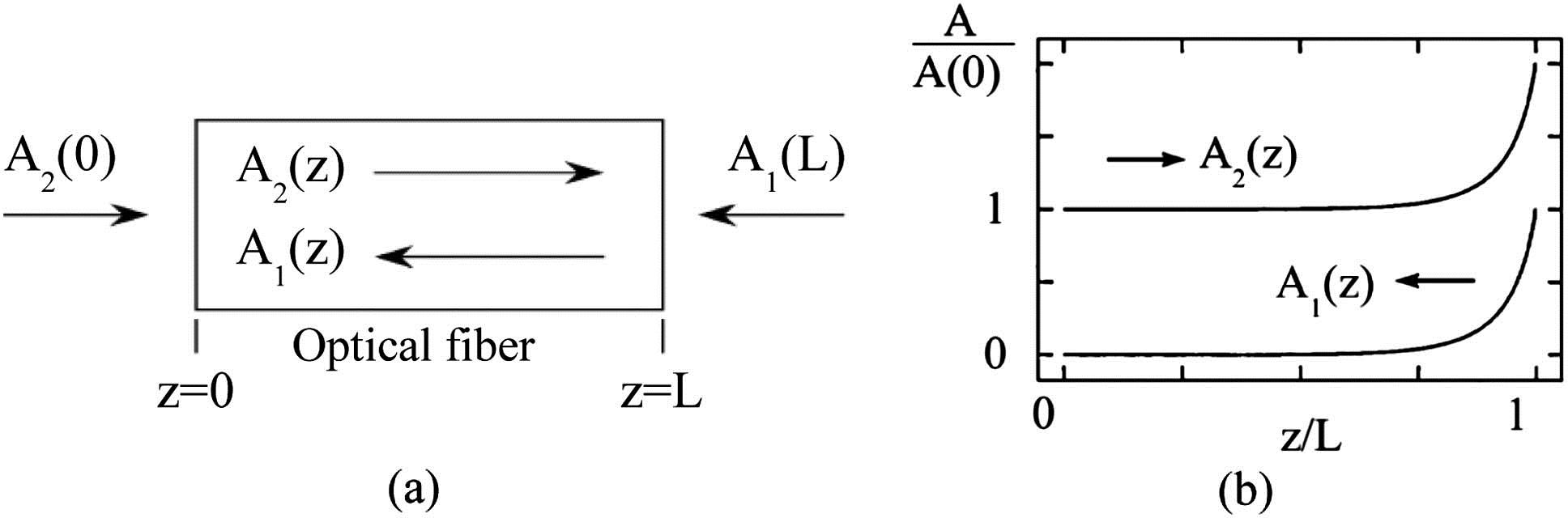
The process of SBS has been studied in a lossless single mode optical fiber, with core radius of 4.1 μm. Attenuation terms have been neglected due to the short fiber lengths inherent in the model. The configuration is composed of a CW launched into one end and a PW launched into the other end of the optical fiber. The schematic arrangement, and intensity distribution, is shown in Fig. 1 below. The pump wave experiences depletion while the probe wave experiences amplification (gain).
Figure 1.(a) Schematic arrangement of SBS in a fiber of length . Pump and probe configuration: —continuous wave, —probe wave. (b) Schematic distribution of the pump and probe intensities during SBS.
The counter-propagating CW and PW induce density variations of the fiber through electrostriction, creating an acoustic grating, or wave, which participates in the SBS interaction [1]. In the slowly varying amplitude approximation, the steady state interaction between the CW and the PW and an acoustic wave (AW) is described by the following system of equations [9]. The system is deemed to operate in the steady-state regime with pulse lengths greater than 10 ns: where is the angular frequency of the AW caused by the interaction of CW and PW, is the complex amplitude of the CW, is the complex amplitude of the PW, is the complex amplitude of the caused by the interaction of CW and PW, is the speed of light, is the density of the fiber, is the electrostrictive constant, is the coordinate along the fiber, is the index of refraction of the fiber, is the speed of sound in the fiber, is the Brillouin linewidth, is the Brillouin frequency defined as , where is the angular frequency of the CW, and is the angular frequency of the PW.
In the above arrangement, the PW input parameters are known only at the beginning of the fiber, i.e., at . Correspondingly, the CW input parameters are known only at the end of the fiber, i.e., at , where is the length of the fiber. Therefore, the boundary conditions for system (1) are as follows: where and are known squared absolute values of the complex amplitudes and , respectively.
The goal is to find analytical expressions for the intensities of the CW and PW. In the dimensionless notation, the system (1) becomes with corresponding boundary conditions The dimensionless variables , , and have been introduced to derive the system (3), as well as the following -coefficients:where is fiber length, is CW intensity, is initial CW intensity, is PW intensity, and is initial PW intensity.
3. SOLUTION
The method used to obtain the dimensionless intensities and yields the following result for the dimensionless intensities of the CW and PW waves: The expression (9) is the gain the PW experiences. Expression (8), rewritten in terms of dimensional intensities and , coincides with the expression for the intensity of the probe wave in [7].
The solution of the system (3) for the intensities (7) and (8) is not complete until an expression for the output intensity of the CW is determined, which corresponds to the root of the transcendental equation [7], shown in expression (10). As such, previously known solutions, being formally analytical, require the numerical solution of expression (10). Therefore, for all practical purposes, previously obtained solutions are better qualified as hybrid solutions (i.e., partly numerical or graphical and partly analytical): The analytical solution of lies in transforming equation (10) into a form suitable for analytical approximation. This form is shown below as expression (11): The transcendental equation of (11) has a single root “” that depends only on two dimensionless parameters and [i.e., ]. Additionally, this root falls within the range [0,1], which represents the range of possible dimensionless output intensities of the CW, giving it a physical significance.
Using Eq. (8), we get the following expression for the output intensity of the PW, assuming is known:
4. ANALYTIC SOLUTIONS
Fully analytic expressions (7) and (8) can only be complete when an analytic expression for is found. Since we are looking for a solution placing no limits on , let us expand the LHS of the equation (11) into a MacLauren series with respect to the variable . If we define, for convenience, and then the corresponding MacLauren series is Thus, Eq. (11) takes a form suitable for finding approximate analytical solutions:
A. Linear Approximation
Keeping only linear terms in Eq. (13), we yield the simplest approximation as follows: If better accuracy is required, the quadratic approximation is in order.
B. Quadratic Approximation
Keeping terms in (13), and after some tedious algebra, we yield the next approximation as follows: where is the output intensity of the CW in the linear approximation, defined in Eq. (14). In a similar way, one can also get the cubic and quartic approximations, which we do not show here due to their complexity.
5. RELATIVE ERROR
To gauge the accuracy of our analytical solutions (14) and (15), we compare them to the numerically calculated solution for the output dimensionless CW intensity. The transcendental Eq. (11) easily lends itself to numerical solution with the use of standard methods of computational physics.
A. Linear Approximation
The relative error is less than 33% in the worst case, on the interval , , as it is shown in Fig. 2 below.
Figure 2.Relative error of linear approximation of 3D parametric model of output CW. , , .
The relative error of the quadratic approximation is 6.5% in the worst case, which is more than three times smaller than the relative error given by the linear approximation.
Notice, however, that except for a limited combination of parameters for which there is an increase in relative error, deemed to be the “worst case,” the relative error in most of the calculations shown in Figs. 2 and 3 is close to 0%. This confirms the utility of the analytic approximations.
6. 3D PARAMETRIC MODEL
An analytic 3D parametric model, attained by plotting the linear approximation solution as a function of dimensionless parameters and , is shown in Fig. 4.
Figure 4.Linear approximation of 3D parametric model of output CW. Dimensionless output intensity of the CW versus dimensionless parameters and . , , , μ, , , , .
As can be seen from Fig. 4, the linear approximation (14) covers the entire range of values of output intensities of the CW [i.e., from weak depletion, to full depletion when ]. In spite of its simplicity, this 3D parametric model is valid in a wide range of combinations of dimensionless parameters and .
Using Eq. (12), a similar 3D parametric model for the output probe intensity is calculated and shown below in Fig. 5.
Figure 5.Linear approximation of 3D parametric model of output PW. Dimensionless output intensity of the PW versus dimensionless parameters and . , , , μ, , , , .
As expected, while the CW experiences depletion, the PW experiences amplification.
7. 3D PARAMETRIC MODEL: SIMILAR AND DISSIMILAR PROCESSES
The 3D parametric model for the output CW intensity allows for the easy interpretation of the effects of pump and pulse powers on the level of CW depletion in the fiber. Parameters of the fiber are described in Figs. 4 and 5, and the range of pump and pulse powers , , correspond to the following range of dimensionless parameters and : ; . This power range models CW depletion from 0%–100%, corresponding to in Fig. 4. For example, restricting the range of pulse power to yields a depletion of 55%–100%. Further changes in pulse power change the level of depletion accordingly. Being a very versatile model, a change in pulse power, parameters of the fiber, or fiber length would alter the restrictions on and , therefore allowing for the “picking and choosing” of the preferred level of depletion for the given fiber. For example, in optical fibers it is often preferable to avoid large depletion, which would require a pulse power of for the parameters given in Figs. 4 and 5.
The study of analytical solutions for the output CW intensity has led us to notice that certain patterns of similarity exist between various amplification processes in each regime, even though each process may be described by different combinations of parameters of amplification. Namely, a point on the 3D parametric model, corresponding to a subset of Brillouin amplification processes, determined by the values of the dimensionless parameters and , is called the representative point. Two Brillouin amplification processes are called similar if they are characterized by the same representative point. Conversely, two Brillouin amplification processes are called dissimilar, if they are characterized by different representative points. The degree of similarity between two Brillouin amplification processes and is determined by the distance between their representative points, a bigger distance indicating a smaller degree of similarity, and vice versa. Figure 4 above shows an example of two similar and two dissimilar processes. In example 1 below, processes and are represented by points and , while process is represented by point , in Fig. 4.
Example 1.
Similar Processes: , , ,
Process A: , , , , , , , , , , , ,
Process B: , , , , , , , , , , , ,
Dissimilar Processes: , , ,
Process A: , , , , , , , , , , , ,
Process C: , , , , , , , , , , , ,
8. APPLICATIONS
A. Fiber Sensing
Classification of the Brillouin amplification processes, in terms of their degree of similarity as described above, may have useful applications in the design of various devices based on Brillouin scattering, such as fiber optic sensors. Indeed, a design specification for a device is likely to require that a certain level of output signal be achieved within a certain margin to ensure normal operation of the device. Practice shows that there often exist severe design and technological constraints for many such devices; therefore, though theoretical considerations may suggest a combination of parameters of the Brillouin amplification process that meets the design specification requirements, this theoretical combination may be impractical, expensive, or simply unavailable technologically. In this case, the 3D parametric model would be useful in finding an alternate combination of parameters that is available technologically, and that either meets the requirements of the design specification or is reasonably close to it. Such a model would allow for the quick and inexpensive attainment of the maximum utility and performance from such a device.
B. Photonic Logic
Another important application is one in photonic logic. In [14], a possible construction of an optical NOT gate utilizing the mechanisms of SBS has been described. To obtain a high switching contrast of 77.6%, such as the one obtained in [14], it is important to find the correct combination of fiber parameters. The initial probe power, , was chosen to be the input signal, and an output CW power, , was taken to be the output signal of the optical gate. The input CW power was taken to be the reference signal, and was held constant at . An input power of 0.1 mW was assigned a logical value of “0,” while an input power of 10 mW was assigned a logical value of “1.” Output powers of 9.0 and 1.33 mW were obtained for the logical inputs “0” and “1,” respectively, yielding the switching contrast of 77.6%. In the configuration described in [14], a SMF-28 fiber was used, of length 350 m, and a 1550 nm laser.
The Brillouin surface can be used to reconstruct this optical gate for any combination of parameters, not only for the ones used in [14]. For example, it is possible to reproduce the optical logic gate of [14] for the SMF-28e fiber, 1310 nm laser, and 1000 m fiber, used in this manuscript, by referring to the Brillouin surface in Fig. 4. From Fig. 4, it is seen that a reference input CW beam of 10 mW corresponds to ; hence all combinations of parameters must be on the parametric curve corresponding to . Furthermore, the output CW power of , corresponding to the “0” output, in turn corresponds to . For the parameters taken in this manuscript, this yields an input probe power of . Likewise, the output CW power of , corresponding to the “1” output, in turn corresponds to . Again, for the parameters taken in this manuscript, this yields an input probe power of . Hence, just by looking at the Brillouin surface in Fig. 4, it is possible to find the combination of parameters of the fiber, to recreate the optical logic gate described in [14]. Of course, the 3D parametric model may also be used to construct an optical gate with a higher switching contrast than the one disclosed in [14], or for different, more practical, input powers.
9. SPECTRAL CHARACTERISTICS
A. Analytical Expressions
The starting point in the analysis of analytical expressions for Brillouin output spectra is the previously derived expressions for the output intensities of the CW: , expressed in Eq. (14), and the PW: , expressed in Eq. (12). Denoting and , the following standard approximations are made: With these approximations in mind, we yield, instead of (14), much simpler expressions: where , .
And Analytical expressions for the full width at half-maximum (FWHM) of the spectra may also be obtained, valid for 0%–100% nonlinearity. For the simplicity of notation, we introduce , and recall that : Using the expressions (7) and (8), we are able to describe the behavior of the CW and PW at every coordinate inside the fiber, and the corresponding output intensity spectra obtained from expressions (17) and (18) above.
Looking at the probe wave spectrum in Fig. 6, we can see that spectral distortion occurs with increasing probe wave power. Energy is transferred from the pump (higher frequency) to the probe wave (lower frequency). A strong probe signal can induce pump depletion [15], since it causes the pump to transfer more energy. However, since , saturation effects occur because there is not enough energy supplied by the pump.
To better demonstrate the correlation between pump depletion and probe spectrum distortion, the is plotted versus pump depletion in Fig. 7 for various probe powers, where FWHM is the full width at half-maximum of the probe spectrum from expression (20), and is the gain of the probe wave from expression (9). The more distorted the probe spectrum, the higher its ratio value will be. Depletion of the pump was calculated using expression (7).
Figure 7.Pump depletion as a function of probe spectral distortion. (mW) = ○ 0.01; ▵ 1.8; × 6.6; ◻ 12.1; ▿ 17.1; + 22.4; * 27.2; ▪ 31.8; ♦ 36.3. , , , , , , , .
As can be seen from Fig. 7, the stronger the probe power, the greater the pump depletion. Consequently, the spectral distortion of the probe spectrum is higher (higher ratio). The Lorentzian shape of the spectrum then becomes flattened and the FWHM increases, as saturation effects begin to become prominent. As such, an output Lorentzian probe wave spectrum (low ratio) is an indication of low pump depletion, while an increase in spectral distortion (high ratio) is symptomatic of an increase in pump depletion and saturation effects.
Pump depletion is detrimental in the field of fiber-optic sensing devices, since it causes a deviation of the peak frequency of the recorded spectrum from the local Brillouin frequency shift, resulting in a systematic error in temperature/strain evaluation [15]. Hence, a Lorentzian probe spectral shape is desired to ensure minimal pump depletion. It is possible to use the 3D parametric surface to avoid parameter combinations, which would lead to such a spectral distortion effect and, instead, choose parameter combinations that would yield an approximate Lorentzian profile. This will be described in more detail in Section 9.B.
B. Transition to a Lorentzian Spectra (Curvature)
As can be seen from Section 9.A, in the nonlinear case, the general expression for the probe wave spectrum (18) does not represent a Lorentzian profile. However, it can be seen from Fig. 6, as well as experimental results (Fig. 10 below), that for certain combinations of parameters, the output PW spectrum is very close, if not indistinguishable, to the Lorentzian spectrum. In this section we will determine the conditions, within a given level of tolerance, for which the output CW and PW spectra have a Lorentzian profile.
Since a purely Lorentzian spectrum is characteristic of linear systems, it is expected to occur for small nonlinearities (i.e., for small , ). Expanding the expressions (17) and (18) into a power series with respect to and , we get the following linear approximations: It can be seen from Eqs. (21) and (22) that the first (linear) term is representative of a Lorentzian profile, (while higher terms distort it). Ensuring that these distortions are much smaller than the Lorentzian term, we require that For a nonlinear phenomenon like SBS, the spectral shape inevitably deviates from the Lorentzian profile as either the pump power (), or probe power () are increased. It can be seen from Fig. 6 that the spectrum becomes flattened quicker than it widens in the onset of spectral distortions. As such, the sharpness of the spectral tip is more sensitive to changes in the spectral shape, as compared to the FWHM of the spectrum. For this reason, we measure the deviation of the spectral shape from the Lorentzian shape by using the relative deviation of the curvature, , of the distorted spectral tip as compared to the Lorentzian spectral tip, according to the following expression: Using the standard definition of the curvature of the plain curve, as well as expressions (17) and (18), respectively, we yield the following expressions for the curvatures of the CW and PW, and , respectively: where , and are defined in Eq. (19). From expressions (21) and (22), we find the curvature of the corresponding Lorentzian profiles (maximum curvature) for the CW and PW, respectively: Given the tolerance , we find the following inequality for a quasi-Lorentzian spectral shape: The range of and values for which the tolerance does not exceed from the Lorentzian curvature is shown in Fig. 8. For clarity, the scales along the and axes are different. A tolerance of 20% cannot be achieved for -values exceeding 0.50, corresponding to a power range of for fiber parameters in Fig. 6, while it is possible to choose any -value, which corresponds to the power range , provided it is coupled to the correct -value.
Figure 8.Shaded area depicts range of and values that yield curvatures within 20% of the Lorentz curvature for both CW and PW spectra.
This reflects the current theory in which weak probe powers are usually utilized for sensing applications, since this is the regime in which a Lorentz-like profile may be achieved. As such, fiber and strain measurements (measurements of the probe wave) are best conducted within the -parameters shown in Fig. 8, provided that other factors, not considered here, do not require otherwise.
10. EXPERIMENT
A. Experimental Setup
The experimental setup is shown in Fig. 9. Two narrow linewidth (3 kHz) fiber lasers operating at 1310 nm are used to provide the pump and probe waves, respectively. The frequency difference is locked by a frequency counter and is automatically swept to cover the Brillouin range. A 12-GHz bandwidth high-speed detector is used to measure the beating signal of the pump and probe waves, providing feedback to the frequency counter to lock their frequency differences. The pump laser is launched into an optical circulator, which passes through into the fiber under test (FUT), which is a 1 km Corning SMF-28e. The probe laser is launched into the FUT, to interact with the pump wave, after which it re-enters the optical circulator.
As can be seen from Fig. 10, the same kind of spectral distortion can be seen in the experimental results as shown in the analytical expression of Fig. 6. For both the experimental and theoretical results, the Lorentzian spectrum is maintained for low depletion (i.e., when ), the intensity drop at resonance is progressively more gradual, and the shape becomes flatter. The second, smaller peak seen at 12,925 MHz is a result of second-order Brillouin scattering effects [16], which are not taken into consideration in this paper.
Accurate analytic expressions have been obtained for Brillouin amplification, describing the intensities of the CW and PW for any coordinate inside the fiber, without any underlying assumptions about the behavior of the pump or probe waves. Among these solutions are (i) the linear approximation which gives a maximum relative error of 33% and (ii) the quadratic approximation which gives a maximum relative error of 6.5%. The relative error for the above analytic solutions quickly decreases to for the majority of parameters.
Additionally, analytic solutions for the output pump and probe spectra have been obtained to good accuracy, as well as an expression for the FWHM. These solutions model a spectral distortion effect, which takes place at high pump depletions and high probe powers, and is confirmed experimentally. In sensing applications, the 3D parametric model may be used to avoid parameter combinations, which yield unwanted spectral distortion effects, such as in distributed sensing where CW depletion is substantial.
The 3D parametric model can also be used to classify the similarity between various Brillouin amplification processes, making it possible to attain the same CW output intensity with a different collection of parameters of the fiber. Such an application has various uses in the field of photonic logic, where reconstruction of optical logic gates for various fiber parameters is required.
[13] L. Thévenaz, S. F. Mafang. Depletion in a distributed Brillouin fiber sensor: practical limitation and strategy to avoid it. Proc. SPIE, 7753A5, 1-4(2011).
Daisy Williams, Xiaoyi Bao, and Liang Chen, "Characterization of high nonlinearity in Brillouin amplification in optical fibers with applications in fiber sensing and photonic logic," Photonics Res. 2, 1 (2014)