


S. Weber, and C. Riconda, "Temperature dependence of parametric instabilities in the context of the shock-ignition approach to inertial confinement fusion," High Power Laser Sci. Eng. 3, 010000e6 (2015)
- High Power Laser Science and Engineering
- Vol. 3, Issue 1, 010000e6 (2015)
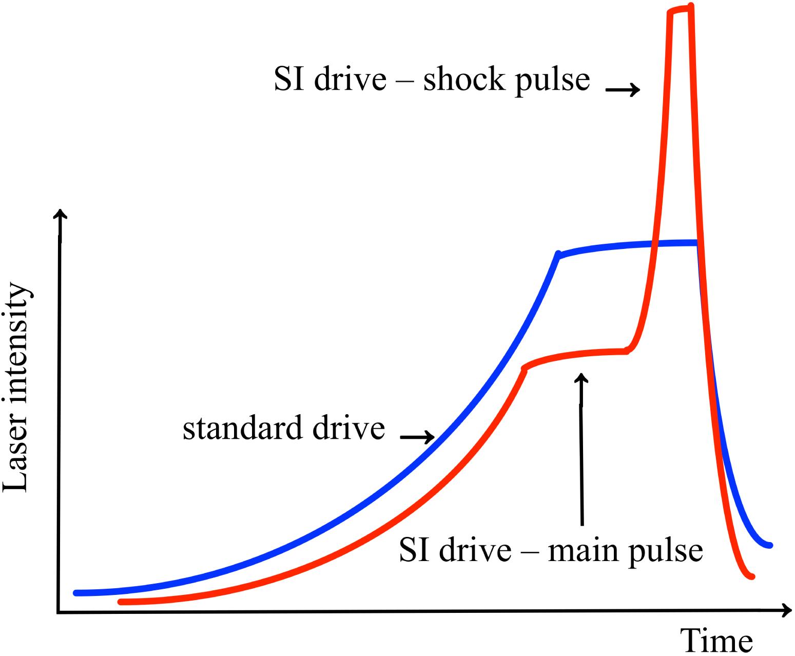
Fig. 1. The temporal evolution of the intensity in the case of conventional drive (blue curve) and SI drive (red curve). In the standard approach to ICF the driver is responsible for fuel assembly and a high velocity,  , for igniting the fuel due to the creation of a hotspot. In the SI scenario the main drive is responsible for fuel assembly but at a lower velocity,
  , preventing ignition. The short high-intensity shock-inducing pulse launched at a later time will reach the fuel at stagnation and ignite it. (Note: the curves in this cartoon drawing are not to scale.)
, for igniting the fuel due to the creation of a hotspot. In the SI scenario the main drive is responsible for fuel assembly but at a lower velocity, , preventing ignition. The short high-intensity shock-inducing pulse launched at a later time will reach the fuel at stagnation and ignite it. (Note: the curves in this cartoon drawing are not to scale.) 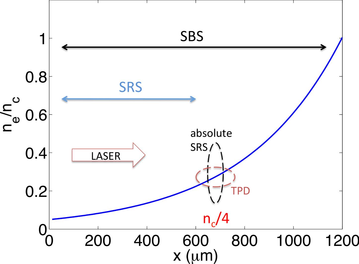
Fig. 2. Localization of the various parametric instabilities in the plasma profile. The figure represents a realistic profile. The one used in the simulations is smaller (see Section 2 ).
Fig. 3. The profiles of the plasma and the incident laser beam. The parameters are given in Section 2 .
Fig. 4. Geometry of the  -vectors involved in the TPD instability. The decay of a photon into two plasmons can be realized in two possible ways while preserving energy and momentum. This particular geometry applies in 2D and helps with the interpretation of the phase space diagrams. In reality, 3D, the number of possible
  -vectors is infinite lying on an asymmetric cone around the laser
  -vector.
-vectors involved in the TPD instability. The decay of a photon into two plasmons can be realized in two possible ways while preserving energy and momentum. This particular geometry applies in 2D and helps with the interpretation of the phase space diagrams. In reality, 3D, the number of possible -vectors is infinite lying on an asymmetric cone around the laser -vector. Fig. 5. Reflectivities ( , i.e., reflected intensity over incident intensity at the centre of the speckle in the transverse direction) for the cases (a) c8, (b) h8, (c) h7 and (d) h9. The curves are ‘filled’ as the laser temporal period is resolved. The blue curve corresponds to SBS-like frequencies, summing the range
  –
– . The red curve corresponds to SRS-like frequencies, summing the range
  –
– . No frequencies are present in the interval
  –
– . Note: the time on the axis refers to the moment the reflected light crosses the boundary of the computational box; as the quarter critical density is located at
  , the light was actually refelected
  earlier.
, i.e., reflected intensity over incident intensity at the centre of the speckle in the transverse direction) for the cases (a) c8, (b) h8, (c) h7 and (d) h9. The curves are ‘filled’ as the laser temporal period is resolved. The blue curve corresponds to SBS-like frequencies, summing the range –. The red curve corresponds to SRS-like frequencies, summing the range –. No frequencies are present in the interval –. Note: the time on the axis refers to the moment the reflected light crosses the boundary of the computational box; as the quarter critical density is located at , the light was actually refelected earlier. Fig. 6. Poynting vector for the case h9 at  .
.
. Fig. 7. Frequency spectra for the cases (a) c8, (b) h9 and (c) a zoom of (b). Note: (a) and (b) are on log scale whereas (c) is on linear scale.
Fig. 8. Two-dimensional Fourier spectra of the electromagnetic field  evaluated in the vicinity of
  for the cases c8 (a, c) and h9 (b, d) taken at times
  (a, b) and
  (c, d).
evaluated in the vicinity of for the cases c8 (a, c) and h9 (b, d) taken at times (a, b) and (c, d). Fig. 9. Poynting vector for the case c8 at  . The ‘hole’ behind the density layer around
  is clearly visible.
. The ‘hole’ behind the density layer around is clearly visible. Fig. 10. Fourier transform of the ion density corresponding to Figure 11 . (a) Case c8 at  , (b) case h8 at
  , (c) case h7 at
  and (d) case h9 at
  . It should be noted that the axes for the various cases differ as the
  -vectors become shorter as the temperature increases.
, (b) case h8 at , (c) case h7 at and (d) case h9 at . It should be noted that the axes for the various cases differ as the -vectors become shorter as the temperature increases. Fig. 11. Ion density near the quarter critical density (located at  . (a) Case c8 at
  , (b) case h8 at
  , (c) case h7 at
  and (d) case h9 at
  . It should be noted that the colour scale used is not the same for each of the four sub-figures in order to enhance the visibility of the structures.
. (a) Case c8 at , (b) case h8 at , (c) case h7 at and (d) case h9 at . It should be noted that the colour scale used is not the same for each of the four sub-figures in order to enhance the visibility of the structures. Fig. 12. The transverse electron phase space as a function of the laser propagation direction for (a) case c8 at  , (b) case h8 at
  , (c) case h7 at
  and (d) case h9 at
  . The time slice for h9 is taken at an early time as the electrons start to recirculate quickly.
, (b) case h8 at
, (c) case h7 at and (d) case h9 at . The time slice for h9 is taken at an early time as the electrons start to recirculate quickly.
|
Table 1. Summary of the simulations. Here,  refers to the laser intensity,
  is the electron plasma temperature. All simulations are at
  , i.e., a laser wavelength of
  . The fully relativistic PIC code emi2D[42] was used for all simulations;
  for all simulations. The reduced intensity case i8 will not be discussed in the text as the results show the same scenario as the corresponding high-intensity case h8.
refers to the laser intensity, is the electron plasma temperature. All simulations are at , i.e., a laser wavelength of . The fully relativistic PIC code emi2D[42] was used for all simulations; for all simulations. The reduced intensity case i8 will not be discussed in the text as the results show the same scenario as the corresponding high-intensity case h8.
|
Table 2. Temperature-dependent occurrence of LPI phenomena. The number of stars gives a rough ‘visual’ interpretation of the strength of the process occurring, with  strongest and
  weakest. The numbers in the columns
  and
and  are calculated from the corresponding Equations (
5 ) and (6 ). The thresholds have to be compared with the laser intensity, which in units of  is 1.2 for all cases. CAV
  cavitation.
strongest and weakest. The numbers in the columns and are calculated from the corresponding Equations ( is 1.2 for all cases. CAV cavitation. 

Set citation alerts for the article
Please enter your email address

© Copyright 2018-2021 | Chinese Laser Press. All Rights Reserved 沪ICP备15018463号-20