
Ling Hong, Haoxu Guo, Xiaodong Qiu, Fei Lin, Wuhong Zhang, Lixiang Chen. Experimental optical computing of complex vector convolution with twisted light[J]. Advanced Photonics Nexus, 2023, 2(4): 046008
- Advanced Photonics Nexus
- Vol. 2, Issue 4, 046008 (2023)
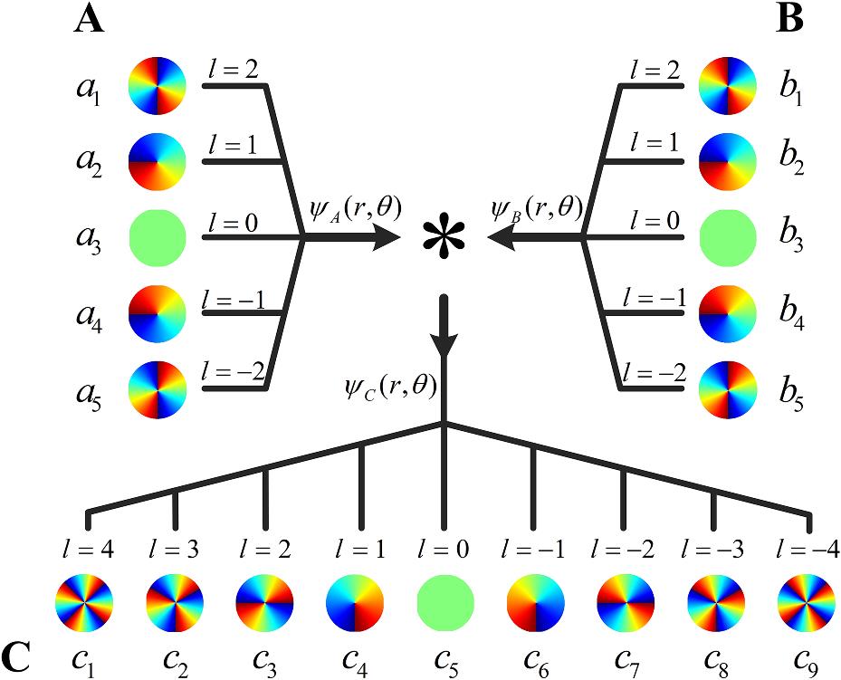
Fig. 1. The schematic diagram of the optical complex vector convolution
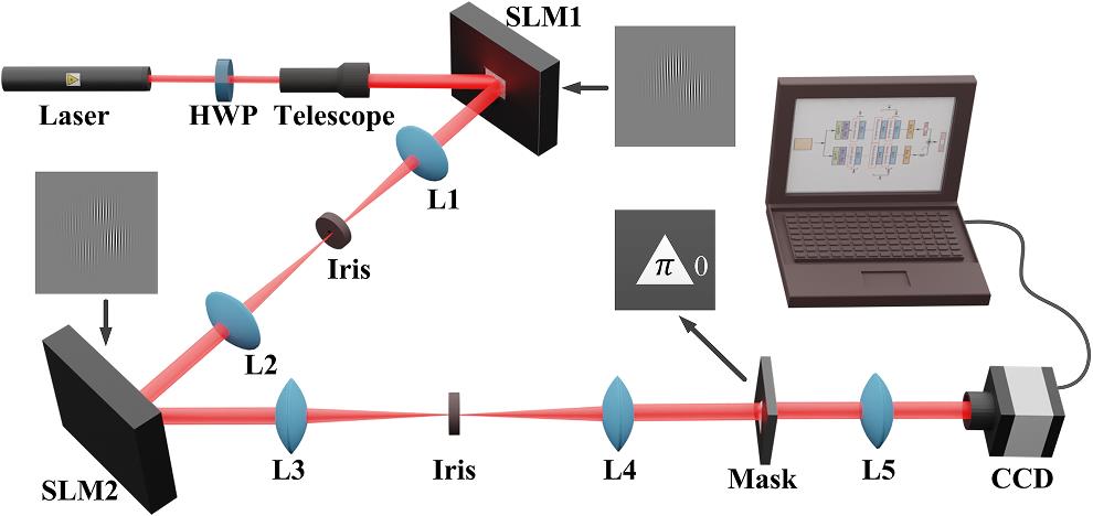
Fig. 2. Schematic of experimental layout for optical computing of complex vector convolution based on OAM eigenstates. HWP, half wave plate; SLM, spatial light modulator; L1, L2, L3, L4, L5, lenses; Mask, a phase triangular object; CCD, camera. Inset, holographic example of encoded complex vector with four OAM states in SLM1 and SLM2.
Fig. 3. Architecture of the residual neural network.
Fig. 4. Complex vector convolution process and experimental results of 7-dimensional OAM state vectors. The input vectors (a)
Fig. 5. The distributions of (a) proximity and (b) relative errors obtained by comparing each experimental predicted output vector with the theoretical output vector for 7-dimensional OAM state vector convolution.
|
Table 1. Average proximity and mean relative error of the output vector from 7-, 9-, and 11-dimensional OAM state vector convolution.

Set citation alerts for the article
Please enter your email address
© Copyright 2018-2021 | Chinese Laser Press. All Rights Reserved 沪ICP备15018463号-20