With the exponential growth of daily data generation in today’s world, the exploration, utilization, and analysis of data require huge energy-efficient computing power.1^,2 However, the demand for computing power has far exceeded the supply of Moore’s Law, and electronic architecture faces fundamental limitations.3^,4 Processors based on traditional electrical methods have hit unsustainable performance growth bottlenecks.5 The industry needs a new technology that can embark on a new journey. Optical computing makes good use of the characteristics of light, such as inherent parallelism, strong anti-interference, and ultrahigh propagation speeds, which show great superiority in processing massive amounts of data and information in parallel.6^–8 Optical interconnects have been already used in practice to help remove the electronic bottlenecks. All kinds of indications show that the photon is the optimal carrier for the next generation of computing power in the post-Moore era.

Among the types of the optical computation, matrix calculation is the most widely used and indispensable basic mathematical operation in information processing. In recent years, the study of photonic matrix calculation has developed rapidly. The theoretical model of optical vector–matrix multiplier, an important step in optical calculation, could be traced back to the work by Goodman in 1978.9 Then, various photonic devices were successfully used in optical matrix calculations, such as the plane light-conversion method,10^–14 Mach–Zehnder interferometric method,15^,16 and wavelength division multiplexing method.17^,18 The first two methods used the coherent light and operated in the whole complex field. Conventional digital electronic computing platforms are incapable of executing truly complex valued representations and operations, while the wavelength division multiplexing method is incoherent superposition of the different wavelengths and is routinely used for real number matrices.5^,19 As photonic networks excel in matrix vector manipulation, artificial intelligence and optical computing are being combined to develop intelligent photonic processors and photon accelerators.20^–25 In particular, based on optical neural networks, an interesting universal optical vector convolution accelerator has been proposed to realize image recognition.25 It is noted that convolution is a useful operation that can be used to blur or sharpen optical images, which plays a crucial role in optical image processing.26 Besides, traditional digital computing platforms show a significant slowdown in implementing algorithms using complex values. Complex numbers are represented by two real numbers, thereby dramatically increasing the source cost of computation.27 However, the ability of optical computation to perform complex-valued arithmetic makes it an excellent tool for solving the digital computing problem. For example, Zhang et al. devised an optical neural chip that implements truly complex-valued neural networks by modulating the phase and magnitude of the light beam.23 To date, the multiple dimensions of light, such as optical wavelength, time, phase, and magnitude, have been fully explored to implement optical vector convolution. It was Allen and coworkers who recognized that the Laguerre–Gaussian (LG) beams with a helical phase front of exp(iℓϕ) carrying a well-defined orbital angular momentum (OAM) of ℓℏ per photon,28 where ϕ is the azimuthal angle and ℓ is the OAM quantum number. Because ℓ is an integer, the OAM state-space is theoretically unbounded. This provides a promising playground for a variety of applications both in the classical and quantum realms.29^–31 However, photonic OAM, as the inherently high-dimensional degree of freedom of photons, remains relatively unexplored in optical computing.

In this paper, we present an effective optical computing protocol for complex vector convolution using coherent superpositions of high-dimensional OAM eigenmodes. Benefiting from the one-to-one mapping relation between OAM eigenmodes and vector elements, our protocol allows the computing results of complex vector convolution to be just the specific OAM spectrum of output light field. In our experiment, we use two cascaded spatial light modulators (SLMs) to prepare suitable OAM superpositions to encode two complex vectors and devise deep-learning strategy with simple-aperture diffraction to measure the complex-valued OAM spectrum, thus accomplishing the optical convolution task. In comparison with other schemes using optical interferometric methods, for complex arithmetic in phase and magnitude, the OAM needs no optical interferometer such that it may robust for implementing complex calculation tasks. In addition, using a phase triangular aperture, we can extract the OAM complex-valued spectrum from the diffraction pattern in the output port to verify our convolution calculation. Our work clearly demonstrates that the OAM can be an alternative path to implement the complex vector convolution. All the classical linear physical dimensions of light can be controlled independently at the same time. Hence, the combination of multiple degrees of freedom can achieve richer optical operation and may prove valuable tools toward practical optical information processing.

Convolution is an important operation in signal and image processing. It is defined as the integral of the product of the two functions after one is reversed and shifted. Considering two vectors of N dimensions, A=[a1,a2,…,aN] and B=[b1,b2,…,bN], their convolution leads to a third vector C=[c1,c2,…,c2N−1], where ck=∑n+m−1=kanbm,k=1,2,3,…,2N−1.(1)

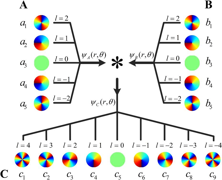
Benefiting from the one-to-one mapping relation between OAM eigenmodes and vector elements, we show that in our protocol the computing results of complex vector convolution may just be the specific OAM spectrum of the output light field. In order to clearly demonstrate our experimental principle, the process of five-dimensional OAM states vector convolution is shown in Fig. 1. Two OAM superposition states, ψA(r,θ)=∑nanEln(r)exp(ilnθ) and ψB(r,θ)=∑mbmElm(r)exp(ilmθ), are composed of five different OAM modes with ln/lm∈{−2,−1,0,1,2}. Each OAM mode carries weight an or bm, corresponding to the OAM spectrum, that can be a complex number to realize the encoding of the two input vectors A=[a1,a2,a3,a4,a5] and B=[b1,b2,b3,b4,b5]. Then, by multiplying the two light fields, the OAM spectrum is redistributed to obtain the output light field ψC(r,θ)=ψA(r,θ)ψB(r,θ). Of particular interest is that the vector C formed by the coefficients of the OAM superposition state ψC(r,θ)=∑kckElk(r)exp(ilkθ) with lk∈{−4,−3,−2,−1,0,1,2,3,4} is exactly the convolution of A and B vectors as described by Eq. (1). Eli(i=n,m,k) represents the amplitude of the beam associated with li, which could be different mode structures, such as LG modes LGpl with the radial index p.32 To keep the integrals of overlap between different modes constant, in our case, we set all the amplitude distributions to the same fixed mode E, which is independent of li. Such a consideration is similar to a perfect vortex.33^,34 In particular, the above process is a one-to-one mapping relation between OAM and vector elements, which does not include algorithms and just uses the transmission property of the light field. Next, we need to extract the OAM complex-valued spectrum C from the output light field ψC(r,θ) to verify our convolution calculation. Traditional methods for obtaining an OAM spectrum are mainly through spatial separation or projection detection of different OAM modes, such as cascade Mach–Zehnder interferometers,35^,36 coordinate transformation,37^,38 digital spiral imaging,39^,40 and multiplane light conversion.41 A concise yet efficient method for precisely and completely reconstructing a high-dimensional OAM complex-valued spectrum remains an open challenge, owing to the difficulties of performing cross-talk-free separation and projection of high-dimensional OAM superposition. In our case, we consider detecting the OAM complex value spectrum without separating each OAM state. Inspired by Hickmann et al., who used a triangular aperture to reveal the topological charge of OAM directly and simply by the diffraction pattern,42 we have recently performed the reconstruction of the OAM complex value spectrum via the machine-learning-assisted recognition of the diffraction pattern.43

Here, we devise deep-learning strategy with simple-aperture diffraction to measure the complex-valued OAM spectrum, thus accomplishing the optical convolution task. Our network contains two paths, trained to obtain the normalized OAM state with the mode weight Ck=ck∑kck*ck and the total strength of the OAM state coefficients ∑kck*ck, respectively. Then, the square root of the latter is multiplied by the former as the final output, and the target state ψC(r,θ) with the mode weight ck is predicted. It should be noted that, unlike the previous work43 using an intensity-only aperture, in our case, we need a phase-only aperture for diffraction to avoid the loss of intensity information due to IC∝∑kck*ck. In addition, our neural network contains two paths, and both based on the residual structure with a regression output, but different in the definition of the loss function. The loss function in path 1 is defined as L1=1−F, where fidelity F=[∑kRe(CP,k*CT,k)]2+[∑kIm(CP,k*CT,k)]2 is usually employed to evaluate the similarity between normalized state used for training with the kth complex-valued amplitude CT,k and normalized predicted state with the kth complex-valued amplitude CP,k. With the decrease of L1, the network gradually finds the mapping between the diffraction pattern and the normalized OAM state and achieves the ability to predict the normalized OAM state vector C/|C|. The loss function in path 2 is defined as L2=|∑kcT,k*cT,k−∑kcP,k*cP,k∑kcP,k*cP,k|,(2)where cT,k and cP,k represent the kth mode weight of OAM state ψC(r,θ), which are used to train the network and are predicted by the network, respectively. In this regard, L2 is used to evaluate the deviation of the total strength of the OAM state coefficients. In this path, we can get the magnitude squared of state vector |C|2. From C/|C| predicted by the two paths, we can easily get our desired vector C as the final output.

The experimental setup is shown in Fig. 2. The desired mode ψA(r,θ) is encoded into the computer-generated holographic mask through complex amplitude modulation of the SLM1. The hologram addressed by the SLM1 is given by32Φ(r,θ)SLM=[Φ(r,θ)Desired+Φ(r,θ)Linear]mod2π×sinc2[1−πI(r,θ)Desired], where Φ(r,θ)Desired=arg[ψA(r,θ)] and I(r,θ)Desired=|ψA(r,θ)|2 are the desired phase and intensity distributions, respectively, and Φ(r,θ)Linear is the phase of the linear grating. With a 4f system consisting of two lenses L1 and L2 (f1=200mm and f2=200mm), a same-sized image of the OAM superposition state ψA(r,θ) is projected onto SLM2 carrying ψB(r,θ). Subsequently, another 4f optical system consisting of two lenses L3 and L4 (f3=150mm and f4=250mm) filter out our desired mode ψC(r,θ)=ψA(r,θ)ψB(r,θ). In the aforementioned process, we have successfully achieved the encoding input of vectors A and B, resulting in the OAM state ψC(r,θ), which carries all the information of the convolution result vector C of vectors A and B. In order to realize the full reconstruction of OAM complex-valued spectrum C, here we prepare a phase triangular object42 to break the OAM conjugate symmetry, as shown in the mask of Fig. 2. The triangular area is π, while the other areas are 0. Diffraction by a phase-type object will not influence the total light intensity of the input field. Then, through lens L5, the diffraction pattern after the object can be obtained. The diffraction patterns recorded by the CCD camera with a resolution of 1024×1024 are appropriately cropped and downsampled to a resolution of 64×64 to match the input parameters of the residual neural network. With the trained residual neural network, the OAM complex-valued spectrum can be obtained from just one CCD-captured diffraction image. In this process, we overcome the problem of indistinguishable intensity patterns between conjugate superposition states through simple-aperture diffraction, thus unlocking the full complex value spectrum reconstruction based on deep-learning strategy via single-shot measurement.

We resize the intensity distributions to 64×64pixels as the input path 1 and path 2. The structure of ResNet is shown by Fig. 3. One 38-layer ResNet is used to analyze the relationship between the normalized OAM state coefficients and the diffraction patterns in path 1, and another 38-layer ResNet is used to analyze the relationship between the total strength of the OAM state coefficients and the diffraction patterns in path 2. A 38-layer ResNet contains 37 convolutional layers with rectified linear unit (ReLU) activation and a fully connected layer. After the first convolution layer with 64 3×3 filters and the average pooling operation, the data are compressed to a feature map of size 32×32×64. Then, the input successively passes through three stages with 64, 128, and 256 filters, respectively. Each stage contains six residual blocks, each of which consists of two 3×3 convolutional layers and an extra shortcut connection. Convolution with a stride of 2 is used for downsampling between stages. The final stage outputs a feature map of size 8×8×256. Subsequently, a global average pooling operation compresses the data to a feature map of size 1×1×256. The network ends in a fully connected layer and regression. Here, we transform the original ResNet into a regression network by replacing the classification output with a regression one. In particular, the fidelity between OAM states is adopted as the loss functions in machine learning, rather than mean absolute error or mean square error in path 1. The loss function of the other path is defined in Eq. (2). Finally, we combine the output of the two paths as the final output to obtain OAM complex-valued spectrum. In the experiment, we obtained 99,999 diffraction patterns. Among them, we selected 80% for training, 10% for validating, and 10% for testing our neural network. Using a commercial consumer-grade computer [GeForce RTX 3060 Laptop Processing Unit GPU and Intel(R) Core(TM) i7-10870H CPU @ 2.20 GHz and 16 GB of RAM, running a Windows 11 operating system, Microsoft], we took roughly 4.5 h to complete the training with 60 iterations. With the trained network, we only needed ∼130ms to reconstruct the OAM spectrum corresponding to a new input diffraction pattern.

It should be noted that the neural network in our work, which assisted in obtaining the entire complex-valued spectrum of OAM, made the process seem more complex than simply performing convolutions through digital computation. We can use other methods to solve this problem. For example, using the multiplane diffraction methods that have successfully achieved spatial separation of high-dimensional OAM,41 our approach toward all-optical computation processing and information extraction based on OAM convolution operation is extremely promising. However, the above method sacrifices phase information during the extraction process and only extracts intensity information. To showcase the principal verification of our work better and more comprehensively, we utilize the neural networks to assist in extracting all information from the complex spectrum of the OAM. We believe that an all-optical sorter for high-dimensional OAM modes, extracting both amplitude and phase information, should be possible soon, which deserves our further research.

At the beginning of the experiment, we randomly generated 99,999 groups of seven-dimensional complex vectors as input data and realized complex vector convolution through the experimental device mentioned above. Then, we obtained 99,999 diffraction patterns. Among them, we selected 80% for training, 10% for validating, and 10% for testing our neural network. The test set contains 9999 input patterns in total, and 9999 groups of convolution results were predicted by the trained network. Taking a set of them as a display, the convolution result C of input vectors A and B is obtained by our experimental setup, as shown in Fig. 4. The pentagram points in the bar are the experimental predicted results. Clearly, the experimental prediction results agree well with the theoretical values, showcasing the ability of optical complex vector–vector convolution.

To quantitatively assess the accuracy of our optical convolution system, we calculate proximity S and relative error Err between the theoretical output vector C and the experimental predicted vector Cp. Here, the proximity and relative error are defined as S=|C·Cp|C||Cp||2 and Err=||C|2−|Cp|2|C|2|. The unit proximity S and the zero relative error Err indicate the perfect convolution results performed by our system. The histogram of Figs. 5(a) and 5(b) shows the statistical distribution of the proximity and relative error calculated from the 9999 experimental images, corresponding to the convolution of seven-dimensional vectors. It is found to be the average proximity Savg∼0.98 with standard deviation ∼0.02, and the mean relative error Errmean∼0.04 with standard deviation ∼0.03.

Moreover, the greater advantage of the OAM over other photonic degrees of freedom is the inherent high-dimensional property, which can be used to encode boundless information in a single photon. To further show the ability of the OAM in the computational area, we also experimentally verify the 9- and 11-dimensional OAM state vector convolution, respectively. And we also obtained the average proximity and the mean relative error as shown in Table 1. From Table 1, as the dimensionality of the state increases, the average proximity decreases, and the mean relative error increases a little bit. The reason is that the experimental conditions are not ideal, such as the imperfect diffraction efficiency of space light modulator with the increase of the OAM dimension, which are incorporated into the training process to set the reconstruction of the OAM complex-valued spectrum. In spite of the imperfect experimental conditions, we can see that all of the average proximity (nearly above 95%) is a good value for vector–vector convolution results.23 In addition, compared with the current optical computing techniques, such as the experimental accuracy of handwritten digit differentiation, which is about 93.39% when using an all-optical diffractive deep neural network architecture,44 we believe the average fidelity of 95% attains the level necessary for practical application. For OAM optical communications,45 the average fidelity of 95% is also considered to be a high level of accuracy.

In our proposed scheme of complex vector convolution based on OAM, the unbounded nature of the OAM state space theoretically allows for the construction of vectors with an infinite number of dimensions. However, the purity of the OAM superposition state preparation and the accuracy of the OAM complex spectrum reconstruction are the main factors affecting the upper limit of the computable vector dimensionality for convolution operations. Further optimization of the system can be considered from the two aspects of OAM generation and detection, such as modifying the diffraction efficiency curve of the SLM46 or improving the accuracy of the image input to the network.

We have proposed, both theoretically and experimentally, a novel approach to computing complex vector convolution based on OAM eigenstates, benefiting from the one-to-one mapping relation between OAM and vector elements through the programmable SLM. To verify the results of the convolution calculation, an interesting deep-learning-assisted platform has been demonstrated. Our results for 7-, 9-, and 11-dimensional OAM state vector convolutions confirm the good performance of the proposed system and clearly demonstrate the OAM can be an alternative path toward implementing the complex vector convolution. It should be noted that our proposed scheme can load the transmission vectors directly without any algorithms. So, it is possible to extend this scheme to two-dimensional matrices or higher-dimensional operations by expanding two dimensions as one-dimensional vectors with blank spacings or using vortex arrays. Therefore, the photon’s OAM can be a universal and potential tool for many classical and quantum computing operating systems and also can be a key building block to process complex computing tasks. Since all the classical linear physical dimensions of light can be controlled independently at the same time, the combination of multiple degrees of freedom can achieve richer optical operation and may prove to be valuable tools toward practical optical information processing.

Ling Hong received her BS degree from Fujian Normal University in 2018. She is currently pursuing her PhD at the College of Physical Science and Technology at Xiamen University.

Wuhong Zhang currently works as an associate professor in Xiamen University at the Department of Physics. He focuses on studying the application and manipulation of light’s orbital angular momentum (OAM). His current research is the application of OAM in quantum optics as well as in quantum computation.

Biographies of the other authors are not available.

References

[3] M. M. Waldrop. The chips are down for Moore’s law. Nature, 530, 144(2016).
[4] M. Lundstrom. Moore’s law forever?. Science, 299, 210-211(2003).
[7] D. A. B. Miller. The role of optics in computing. Nat. Photonics, 4, 406-406(2010).
[10] Y. Chen. 4f-type optical system for matrix multiplication. Opt. Eng., 32, 77-79(1993).
[27] A. Yadav et al. Representation of complex-valued neural networks: a real-valued approach, 331-335(2005).
[34] P. Li et al. Generation of perfect vectorial vortex beams. Opt. Lett., 41, 2205-2208(2016).
[39] L. Torner, J. P. Torres, S. Carrasco. Digital spiral imaging. Opt. Express, 13, 873-881(2005).
[41] N. K. Fontaine et al. Laguerre–Gaussian mode sorter. Nat. Commun., 10, 1865(2019).
Set citation alerts for the article
Please enter your email address
© Copyright 2018-2021 | Chinese Laser Press. All Rights Reserved 沪ICP备15018463号-20