Retrieval of Cn2 profile from differential column image motion lidar using the regularization method

Zhi Cheng; Fengfu Tan; Xu Jing; Feng He; Lai’an Qin; Zaihong Hou

doi:10.3788/COL201715.020101

Abstract

We develop a regularization-based algorithm for reconstructing the

C_{n}^{2}

profile using the profile of Fried’s transverse coherent length (

r_{0}

) of differential column image motion (DCIM) lidar. This algorithm consists of fitting the set of measured data to a spline function and a two-stage inversion method based on regularized least squares QR-factorization (LSQR) in combination with an adaptive selection method. The performance of this algorithm is analyzed by a simulated profile generated from the

{HV}_{5 / 7}

model and experimental DCIM lidar data. Both the simulation and experiment support the presented approach. It is shown that the algorithm can be applied to estimate a reliable

C_{n}^{2}

profile from DCIM lidar.

Knowledge of the optical turbulence profile becomes a key issue in wide-field adaptive optics (WFAO) systems^[1,2], free-space optical (FSO) communication^[3,4], and laser beam propagating through the atmosphere^[5,6]. Several approaches have been proposed to measure the $C_{n}^{2}$ profile. The commonly used methods are the radiosonde balloon method^[7], SCIDAR (scintillation detection and ranging)^[8], SLODAR (slope detection and ranging)^[9], MASS (multiple aperture scintillation sensor)^[10], and lidar methods including differential image motion (DIM)^[11] and differential column image motion (DCIM)^[12,13]. Compared with other methods, lidar can measure the turbulence profile in different paths (i.e., horizontal path and slant path) based on active light detection, which makes it enjoy better application prospects.

DCIM lidar^[12] is a recent atmospheric turbulence monitor for sensing real-time vertical profiles of Fried’s transverse coherent length ( $r_{0}$ ). DCIM lidar is capable of obtaining the $r_{0}$ values of different altitudes simultaneously via imaging the differential column onto a CCD, which is superior to DIM lidar time-sharing measurement of the atmospheric coherent length at different altitudes. However, DCIM lidar aims to extract the real-time vertical distribution of the atmosphere refractive structure constant $C_{n}^{2}$ from $r_{0}$ profiles, which involves an inverse problem analogous to DIM lidar. In DIM lidar, slope inversion based on the first derivative has been proposed to avoid a nonphysical solution^[14], but the first derivative may be more sensitive to measurement noise and this algorithm does not perform well currently in free atmosphere. Although $C_{n}^{2}$ profiles based on the generalized Hufnagel–Valley model have been restored from DCIM Lidar, the retrieval method is limited by the a prior turbulence model without universality^[15]. Consequently, it is of particular importance to develop a more efficient, trustworthy, and generalized inversion algorithm used for DCIM lidar.

In this Letter, an algorithm using a regularization technique to restore the $C_{n}^{2}$ profile from DCIM lidar is reported. The algorithm allows accurate and rapid convergence based on a two-stage reconstruction method that enhances immunity to the presence of noise and does not require an initial estimation of the $C_{n}^{2}$ profile. The first stage uses a regularized least squares QR-factorization (LSQR) method to retrieve the general shape of the $C_{n}^{2}$ profile. The second stage is related to an adaptive selecting algorithm to get the stable solution of the final $C_{n}^{2}$ profile. Theoretical analysis, computer simulations, and experiments will be presented to illustrate the efficiency of this algorithm.

Sign up for Chinese Optics Letters TOC. Get the latest issue of Chinese Optics Letters delivered right to you！Sign up now

The relationship between the measured $r_{0}$ from DCIM lidar and $C_{n}^{2}$ can be written as $r_{0} (H) = {[0.423 k^{2} \int_{0}^{H} C_{n}^{2} (h) {(1 - h / H)}^{5 / 3} d h]}^{- 3 / 5},$ (1)where $r_{0}$ , $k$ , $H$ , and $C_{n}^{2}$ are Fried’s transverse coherence length, wavenumber, the beacon altitude, and the refractive structure constant, respectively.

For each experimental point $H_{j}$ ( $j = 1, \dots, M$ , $M$ is the number of experimental data points), Eq. (1) can be written as $r_{0} {(H_{j})}^{- 5 / 3} = 0.423 k^{2} \sum_{i < M} C_{n}^{2} (h_{i}) {(1 - h_{i} / H_{j})}^{5 / 3} Δ h_{i} .$ (2)

Equation (2) can be converted into a typical Fredholm integral equation of the first kind. The linearity of the direct problem can be described by $y = A x + ε,$ (3)where $y$ is the measured DCIM lidar data of size $M \times 1$ , $A$ is an $M \times N$ lower triangular matrix, $x$ is an $N \times 1$ vector representing the $C_{n}^{2}$ profile to be determined, and $ε$ denotes the measurement noise.

The discretized Fredholm equation is severely ill posed^[16], even an extremely small amount of noise $ε$ can give rise to significant errors in the estimate of $x$ . Moreover, the integral kernel ${(1 - h / H)}^{5 / 3}$ of Eq. (1) is almost equal to 0 when $h$ is close to $H$ , enhancing the ill-conditioning of $A$ . Therefore, the standard matrix methods cannot be used in a straightforward manner to compute a meaningful solution.

Regularization is the most frequently used method to solve the ill-posed and ill-conditioned problem. The cost function minimized by the regularization technique using a Tikhonov method can be expressed as^[17] $\min_{x \in R^{n}} ({‖ y - A x ‖}_{2}^{2} + λ {‖ L x ‖}_{2}^{2}),$ (4)where $L$ is the regularization matrix, and the regularization parameter $λ$ should be chosen carefully to balance the error due to measurement noise and regularization. In our work, $L$ is chosen as the first discrete derivative operator rather than the identity to limit rough oscillations due to noise.

In this Letter, as $A$ is a lower triangular matrix and ill-conditioned, we develop a two-stage reconstruction method. The first stage of the reconstruction is conducted by an iterative regularization method based on the LSQR^[18,19] method. The method is suitable for calculating sparse matrices’ usage of the Lanczos bidiagonalization process. Furthermore, LSQR is a more rapid and efficient method performing the regularization effect, where the iteration number is an equivalent of the regularization parameter $λ$ . A reasonable choice for the convergence condition is the optimal iteration number, which can be determined by the L-curve criterion^[20]. In terms of our solution, it is found that 20–30 iterations are sufficient to converge using the L-curve criterion.

However, the first-stage retrieval will contain unwanted fluctuations induced by the noise in the DCIM data. Therefore, it is necessary to implement the second stage to smooth out the artificial oscillations.

In the second stage, an adaptive selecting algorithm is proposed to remove the large oscillations. As the restored profiles from the LSQR algorithm can acquire the global feature of the theoretical profile with repeatable oscillations, the peaks and valleys of the oscillations are then used to analyze the suitable inversion value. The adaptive selecting algorithm consists of the following four steps: (1) detect all the peaks and valleys in the retrieved profile; (2) revise the unreasonable peaks and valleys according to adjoining peaks and valleys; (3) calculate the corresponding median $C_{med} = (C_{peak} + C_{valley}) / 2$ ; (4) select the retrieved value close to median as the final output.

Spatial resolution is a concern involved in the reconstruction of turbulence profile. The spatial resolution in our method is determined by the two stage retrieval. In the first-stage retrieval, the spatial resolution of the turbulence measurements can be designed reasonably according to variation characteristics of $r_{0}$ and atmospheric subdivision. However, after the second-stage procedure, the spatial resolution does not remain constant in the corresponding layer since the larger oscillations of $C_{n}^{2}$ are filtered adaptively. Nevertheless, the variable spatial resolution does not affect the whole turbulence distribution.

Prior to the reconstruction, the measured $r_{0}$ data need to be fitted by an appropriate spline function in consideration of two principle reasons. First, the random noise may easily lead to $r_{0}$ values larger at high altitudes than those at low altitudes since the optical turbulence of the ground layer makes a significant contribution to $r_{0}$ . As a result, negative values of $C_{n}^{2}$ will be produced. Second, the spline function enables us to use arbitrary data in the spline curve, thereby enlarging the range of the measured data used to carry out the inversion. However, we do not employ the $r_{0}$ values at an altitude higher than 15 km. (i) The max detected altitude value of the lidar is between 12 and 15 km, depending on our present transmitted energy of the laser and signal-to-noise ratio. (ii) The variation of $r_{0}$ is very little at the altitudes above 15 km; a small quantity perturbation of $r_{0}$ may result in a huge error of $C_{n}^{2}$ . A slightly modified spline function of DIM^[14] after some trials is exploited to fit $r_{0}$ values of DCIM $r_{0} = {(a_{1} h / (h + b_{1}) + a_{2} h / (h + b_{2}))}^{- 3 / 5},$ (5)where the unit of $r_{0}$ is centimeters. In order to avoid local minima, the four fitting parameters $a_{1}$ , $b_{1}$ , $a_{2}$ , $b_{2}$ are determined by a genetic algorithm.

Simulation is performed to test the accuracy of the recovery of the profile generated from the ${HV}_{5 / 7}$ model. The ${HV}_{5 / 7}$ model represents a typical turbulence strength distribution in altitude of midlatitude meteorology to which the DCIM lidar is now mainly applied. We first use the ${HV}_{5 / 7}$ model to compute the true $r_{0}$ at different altitudes consistent with the measurement data from the DCIM lidar. Random Gaussian noise with a zero mean and 5% variance is added to the true $r_{0}$ as a measurement error. These noisy $r_{0}$ values are then analyzed with the algorithm.

Note that spline curve can smooth noise very well, although it cannot eliminate noise absolutely, which will lead to the smoothed data being higher or lower than the real data. Therefore, in order to illustrate the effectiveness of the retrieval method, two typical simulation cases will be discussed when the random noise is added to the measurement data: (1) a majority of the fitted data are smaller than the theoretical data; (2) a majority of the fitted data are larger than the theoretical data. The simulated results are given in Figs. 1 and 2, respectively.

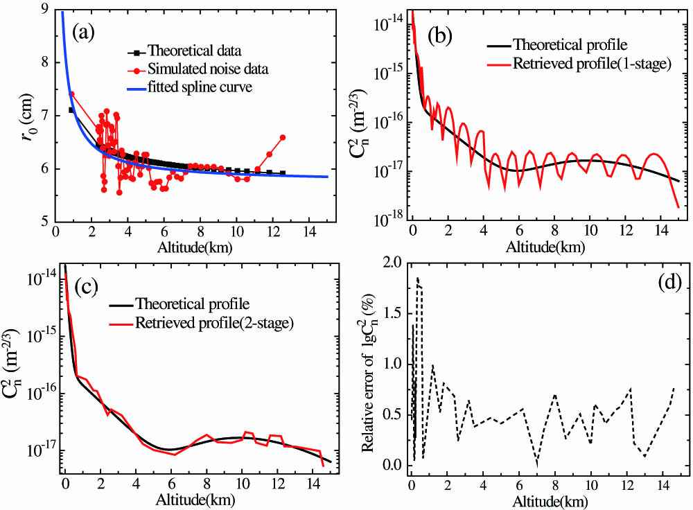
Figure 1.Results of spline curve fitting and two-stage retrieval of a $C_{n}^{2}$ profile for simulated noisy $r_{0}$ values mostly lower than the theoretical data: (a) spline curve fitting with 5% Gaussian noise; (b),(c) the first and second stage of the retrieval, (d) relative error of $\lg C_{n}^{2}$ on the inversion.

A typical noisy $r_{0}$ profile, along with the theoretical $r_{0}$ data and smoothed curve, are presented in Fig. 1(a). From Fig. 1(a), we can see that the simulated data are randomly distributed by 5% Gaussian noise. For the current detection altitude range of 0.8–12.8 km, the smoothed curve is mostly lower than the theoretical one. The restored profile from the noisy data after fitting are shown in Fig. 1(b), noting that the first stage of the reconstruction is able to perserve the bump feature and the whole tendency of the real profile against the error. However, the oscillations in the $C_{n}^{2}$ profile frequently occur with the standard LSQR algorithm. Fortunately, the second stage algorithm can well smooth out the larger fluctuations of the $C_{n}^{2}$ profile derived from the first stage in which the relative error between the input and recovered $\lg C_{n}^{2}$ profile is within 2%.

The simulation process of Fig. 2 is similar to Fig. 1, however, there is a large difference in the input observable quantity. In Fig. 2(a), most of the simulated noise data are higher than the theoretical data. Moreover, the input $r_{0}$ high-altitude values have a larger error than those of Fig. 1(a). In this case, the restored profile using the two-stage algorithm still achieves reasonable values despite some slightly larger fluctuations than those in the first simulated case in the high-altitude turbulence.

Figure 2.Results of spline curve fitting and two-stage retrieval of a $C_{n}^{2}$ profile for simulated noisy $r_{0}$ values mostly higher than the theoretical data: (a) spline curve fitting with 5% Gaussian noise; (b),(c) the first and second stage of the retrieval, (d) relative error of $\lg C_{n}^{2}$ on the inversion.

However, each simulated case is different since the noise is added randomly. The simulation results described above are only two typical cases of simulation samples.

To provide a further illustration of the efficiency of the method, the procedure was conducted in 30 successive cases to compute the mean restoration and root-mean-square error (RMSE) for error analysis. It takes approximately 2.5 s to deduce the final $C_{n}^{2}$ profile for each run. The RMSE represents the residual between the restored and true profile defined as $RMSE (h_{j}) = {(\frac{1}{N} \sum_{i = 1}^{N} {(C_{n_{restored}}^{2} (h_{i j}) - C_{n_{true}}^{2} (h_{i j}))}^{2})}^{1 / 2} .$ (6)

In Fig. 3, we see that the two-stage algorithm permits a good reconstruction at low and high altitudes with smaller oscillations. The RMSEs errors decrease smoothly in the 0–1 km altitude range. For all levels above 1 km, the RMS errors are randomly distributed and less than $10^{- 16}$ .

Figure 3. $C_{n}^{2}$ profile retrieval with the error bars and corresponding RMSEs based on the 30 profiles in the simulation set. The red line represents the average retrieval values of the 30 profiles. The blue line (error bars) is the standard deviation of the 30 profiles.

The signal-to-noise ratio (SNR) is presented in Fig. 4 to evaluate the effectiveness of the proposed method. The SNR equation used can be described as $SNR (h_{j}) = 10 \lg (P_{s} / P_{n}) = 10 \lg (\sum_{i} {(\lg C_{n_{true}}^{2} (h_{i j}))}^{2} / \sum_{i} {(\lg C_{n_{restored}}^{2} (h_{i j}) - \lg C_{n_{true}}^{2} (h_{i j}))}^{2}),$ (7)where $P_{s}$ is the signal power and $P_{n}$ is the noise power. The true $\lg C_{n}^{2}$ is taken as the pure signal without noise and the restored $\lg C_{n}^{2}$ is taken as noisy signal. As the $C_{n}^{2}$ measurements in the real experiments have probably 1–2 orders of deviation from the true values, to avoid the negative SNR, we use $\lg C_{n}^{2}$ rather than $C_{n}^{2}$ .

Figure 4.SNR curve based on the 30 profiles in the simulation set.

From Fig. 4, we see that the range of the SNR is 32–48 dB with a random distribution for different detection altitudes. The SNR is higher in the near surface atmospheric boundary layer and lower at the isolated layer (5–7 km) and near the tropopause (13–15 km).

To demonstrate the validity of this inversion technique experimentally, the DCIM lidar instrument was installed in Hefei on November 9–12, 2015. The transmitter system was developed around an Nd:YAG laser with a 550 nm wavelength. A Cassegrain telescope of 3.7 m focal length was adopted as a receiver whose baseline separation from the transmitter is 4 m. The pupil mask with two 0.12 m diameter subapertures separated by 0.235 m (center to center) was placed at the entrance pupil of the telescope. The CCD of $24 μm \times 24 μm$ pixel size is projected onto the pupil plane. A set of 1000 image frames are acquired to calculate one $r_{0}$ profile. In our present temporal sampling method, one $r_{0}$ profile can be obtained every 20 s, and the single operation time of the inversion algorithm is 2.5 s. Therefore, the final temporal resolution of the turbulence measurements is 22.5 s.

The $r_{0}$ profiles measured with the DCIM lidar for three typical time periods are given in Fig. 5. Three $r_{0}$ profiles represent weak, moderate, and strong turbulence conditions, respectively. It is noted that the $r_{0}$ profile varies little with stronger turbulence. The presented subfigure is to illustrate the random fluctuation of atmospheric turbulence since it is not obvious in the original figure. The fitted spline curve can smooth the random perturbations effectively in different turbulence conditions, preserving the whole tendency of the original profiles.

Figure 5.Example of the measured $r_{0}$ profile with a fitted spline curve (the red, dark yellow, and dark cyan curve) at three typical time periods.

A comparison between the $C_{n}^{2}$ profiles from the DCIM lidar and a radio-sounding balloon is shown in Fig. 6. Each individual profile is determined from the DCIM lidar with an update rate of 22.5 s. The radio-sounding balloon requires 2 h to measure the $C_{n}^{2}$ value from the ground level up to 30 km. The balloon profile shown only contains $C_{n}^{2}$ values between the ground and 15 km for the purpose of comparison with the DCIM lidar profiles. Despite the fact that the two instruments, DCIM lidar and radio-sounding balloon, use completely different principles (image motion and temperature fluctuation, respectively), their results coincide with each other in different turbulence conditions. In Fig. 6(a), the two $C_{n}^{2}$ measurements decrease with random fluctuations, which appear as larger fluctuations between the ground and 4 km as well as 6 and 15 km. Both instruments detect two main turbulence layers, as shown in Fig. 6(b). The weaker turbulence layer is found at approximately 2 km, and a stronger turbulence layer is detected at approximately 8 km. In Fig. 6(c), both the profiles indicate the weakest turbulence at 4 km and a small bump at approximately 10 km. The simultaneous measurements also indicate that the atmospheric optical turbulence near the ground has significant changes with time that may be due to the complicated change features of the underlying surface, but the high-altitude turbulence is relatively stable. The results of the two instruments are in reasonably good agreement, considering that the instruments measured $C_{n}^{2}$ at slightly different times and places. Therefore, the effectiveness of the retrieval method is confirmed experimentally.

Figure 6.Comparison of $C_{n}^{2}$ profiles using the DCIM lidar and radio-sounding balloons at three typical time periods corresponding to Fig. 5.

In order to further quantify the comparisons, using the radio-sounding balloon measurements as reference, Figs. 7 and 8 show the relative errors and the SNR of the DCIM lidar. In Fig. 7, the relative errors are within 11% at three typical time periods. For altitudes above 3 km, the relative errors are less than 4%. Different temporal resolutions of the two instruments and the rapid change of the underlying surface lead to larger errors near the ground. For Fig. 8, the SNR is mainly distributed in the 10–35 dB range. The higher values of SNR mean a better agreement of the two instruments. It is noted that the results of Figs. 7 and 8 only indicate the comparisons between DCIM lidar and radio-sounding balloons, which do not demonstrate the actual error analysis compared with the true values because the balloon measurements also contain experimental errors. However, more efficient experiment comparisons near the ground should be worked on in future.

Figure 7.Relative errors between the DCIM lidar and radio-sounding balloons corresponding to Fig. 6.

Figure 8.SNR of the DCIM lidar at different altitudes corresponding to Fig. 6 (assuming the radio-sounding balloon measurements are pure signals).

In conclusion, we present an algorithm that combines spline function smoothing and a two-stage retrieval method for retrieving the $C_{n}^{2}$ profile from the ground level up to 15 km with DCIM lidar. The algorithm does not require a prior information of the $C_{n}^{2}$ profile and can be computed very quickly. Furthermore, the algorithm can estimate nonlinear spatiotemporal variation features of atmospheric turbulence effectively. The validity of the algorithm is formally verified by both simulation and experiments. The results show that the technique can recover a reliable $C_{n}^{2}$ profile in the presence of noise. The algorithm can also be applied to DIM lidar and other applications using the profile of $r_{0}$ or the variance of angle-of-arrival fluctuations to estimate the $C_{n}^{2}$ profile. Future investigations are needed to reduce the noise contributions of $r_{0}$ profiles to improve the retrieval precision and quantify the spatial resolution of the $C_{n}^{2}$ profile.