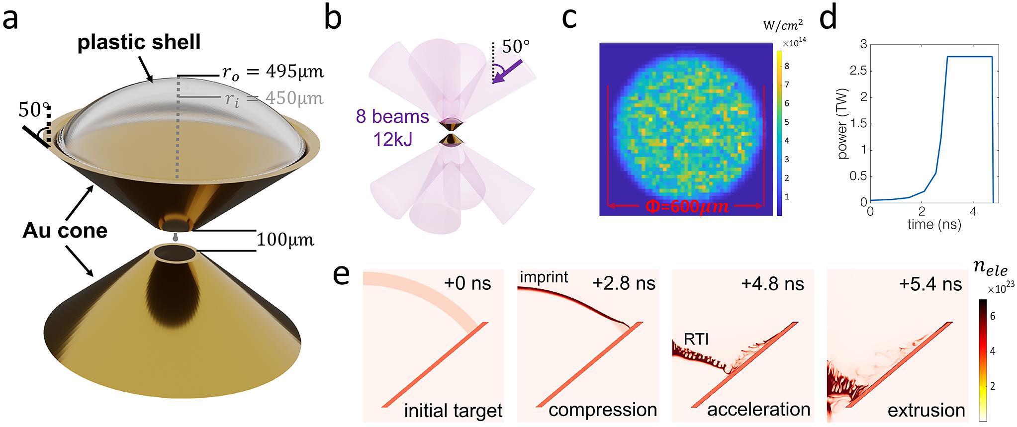
Fig. 1. (a) Schematic of the DCI target. (b) Schematic of the incident laser beams. (c) Power intensity of a single laser spot with inhomogeneous ‘speckle’ feature. (d) An isentropic pulse shape used in the example simulation to show (e) the density distribution at four DCI implosion stages: initial target, compression, acceleration and extrusion. This simulation is conducted in cylindrical geometry and only resolves half of the upper-cone.

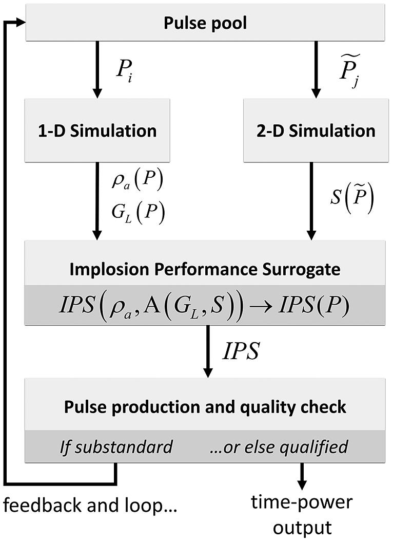
Fig. 2. Pulse shape designer workflow, where the primary goal is to maximize the implosion performance surrogate.

Fig. 3. (a) The pulse shape is decomposed into a finite number of nodes. The example pulse is marked with node power and node timing . Changing the node values generates many other pulse shapes in the same pulse space, as shown by the grey lines. (b) Implosion density and pressure profile of the example pulse at +6 ns. Fitting these profiles to obtain the RTI growth parameters. (c) Calculated RTI growth multiplier of the example pulse.

Fig. 4. (a) The IPS mesh shape, plotted against areal density and perturbation amplitude . (b) Six consecutive optimization batches, each batch containing 2000 pulse samples; complete optimization uses six batches. The left-hand axis shows the batch-averaged IPS score and the right-hand axis shows the pulse space fraction occupied by each batch.

Fig. 5. (a) Illustration of a new pulse point and its distance to the center pulse points. (b) Imprint density of the c9 center pulse. (c) Seed spectrum interpolation for the new pulse. (d) Instability amplitude of the new pulse, with seed correction, without seed correction and the 2D simulation amplitude. (e) Correlation between the interpolated seed spectrum and the 2D simulated spectrum. (f) Dominant mode in the interpolated spectrum and the 2D simulated spectrum.

Fig. 6. Implosion simulation of (a)–(c) the baseline pulse, (d)–(f) the designer-optimized acceleration pulse and (g)–(i) the designer-optimized two-picket pulse. The first row of the figure shows the respective pulse shapes and 1D implosion streamlines. The second row shows the shell’s density at two-thirds and one-third of its initial radius. The third row is the adiabat of the shell at one-third of its initial radius.

Fig. 7. (a) Time evolution of , the distance between the ablation front and the critical surface. (b) Time evolution of the fuel adiabat . The horizontal axis is the laser energy delivered; only the first 2 kJ energy is plotted to clearly show the pickets.

Fig. 8. (a) Pulse shapes when 5% perturbation is added to the optimal two-picket pulse. (b) Eigenvalues of the IPS Hessian matrix. (c), (d) Pulse shapes and implosion streamlines after perturbation along the first and second eigenvectors. The dashed lines are the reference unperturbed pulse shapes.

Fig. 9. Optimized pulse series with and without imprint seed correction. (a) The best pulse in each series is shown with bold lines; the top 10 pulses in each series are shown with translucent lines. (b) Imploding shell density of the best pulse in the uncorrected series, taken at one-third and two-thirds of its initial radius. (c) Areal density perturbation of the two best pulses, where is the fuel polar angle. (d) Center-of-mass perturbation spectrum of the two best pulses.