
Huai-Qian LI, Ming-Hui YANG, Liang WU. High localization accuracy 3D object detection in active millimeter wave holographic images[J]. Journal of Infrared and Millimeter Waves, 2021, 40(6): 870
- Journal of Infrared and Millimeter Waves
- Vol. 40, Issue 6, 870 (2021)
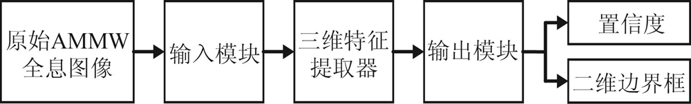
Fig. 1. The structure of our proposed 3D concealed object detector for AMMW holographic images
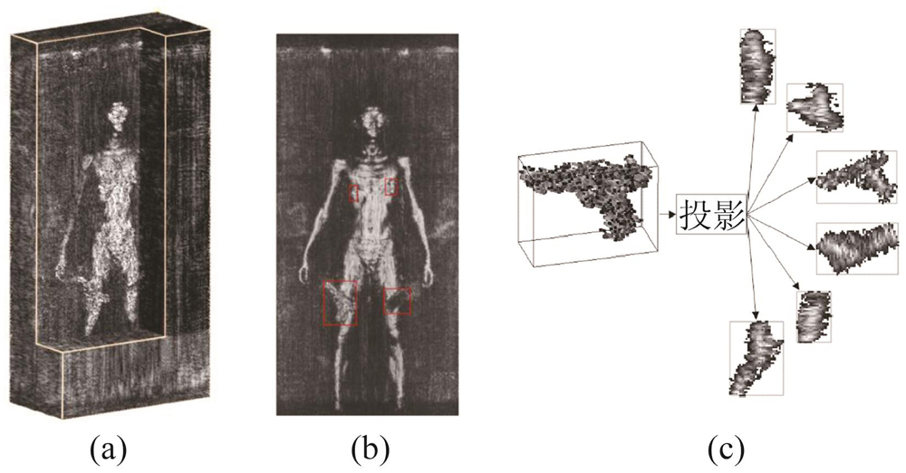
Fig. 2. Projection of the AMMW holographic image (a) AMMW holographic image, (b) the resulting 2D front view of performing projection along the Z axis of the holographic image in Fig. 2(a), (c) the shape and size changes caused by projecting a 3D object into 2D views
Fig. 3. The structure of our proposed input module
Fig. 4. The distribution of the number of points in the bounding box in 3D point clouds and 2D front images
Fig. 5. The structure of our proposed 3D feature extractor
Fig. 6. The structure of our proposed output module
Fig. 7. Comparison of localization and detection performance for different networks (a) Recall as a function of IOU threshold, (b) PR curve under IOU = 0.5
Fig. 8. Qualitative detection results of different networks, where the red bounding boxes denote the ground-truth, and the yellow bounding boxes denote the predicted results (a)-(d) Our proposed method, (e) RPN, (f) Faster RCNN, (g) RetinaNet, (h) TridentNet
Fig. 9. F1-score under different thresholds of the confidence
|
Table 1. Details of convolutional layers of the 3D feature extractor
|
Table 2. Comparison of the AP with different network structures
|
Table 3. Comparison of detection performance on different Networks

Set citation alerts for the article
Please enter your email address
© Copyright 2018-2021 | Chinese Laser Press. All Rights Reserved 沪ICP备15018463号-20