Optical image processing using acousto-optic modulators as programmable volume holograms: a review [Invited]

Yaping Zhang; Houxin Fan; Ting-Chung Poon

doi:10.3788/COL202220.021101

Abstract

Bragg processing using a volume hologram offers an alternative in optical image processing in contrast to Fourier-plane processing. By placing a volume hologram near the object in an optical imaging setup, we achieve Bragg processing. In this review, we discuss various image processing methods achievable with acousto-optic modulators as dynamic and programmable volume holograms. In particular, we concentrate on the discussion of various differentiation operations leading to edge extraction capabilities.

Keywords

acousto-optics edge extraction optical image processing volume gratings

1. Introduction

Standard coherent optical image processing employs a Fourier plane in a 4−f system^[1]. Various image processing operations are accomplished by the modification of the pupil in the Fourier plane. An interesting alternative image processing technique can be performed when we place a thick hologram near the object in an optical imaging setup^[2,3]. Angular selectivity of volume holograms through Bragg diffraction provides the selection of spatial frequencies. We call such a technique Bragg processing. Edge extraction is one of the most important image operations in image processing^[4,5]. S. Case was the first, to the best of our knowledge, to demonstrate optical edge extraction using Bragg processing^[3]. Balakshy pointed out the possibility of using acousto-optic interaction to perform spatial filtering in 1984 and recently presented a short survey on the use of acousto-optics for optical wavefront visualization^[6,7]. Xia et al. for the first time, to the best of our knowledge, demonstrated experimental Bragg diffraction image edge extraction and pioneered image processing in an imaging system with an acousto-optic modulator (AOM) as a programmable volume hologram^[8]. The system provides real-time programmable tuning of spatial transfer functions by various parameters of the AOM. Since then, a variety of optical systems using acousto-optic Bragg processing for edge extraction have been reported. Banerjee et al. employed two AOMs aligned along the $x$ and $y$ directions to achieve mixed partial derivatives^[9]. Cao et al. employed two cascaded AOMs to achieve second-order partial derivatives^[10]. The tandem arrangement of two AOMs has been investigated for expanding the possibilities of using Bragg diffraction for high frequency modulation of optical beams^[11,12]. To develop more and diversified spatial-filtering operations, Banerjee et al. also investigated techniques to compute spatial transfer functions under a variety of physical situations^[13]. Davis and Nowak performed operations similar to those obtained with both the fractional Hilbert transform and fraction derivative spatial-filtering operations^[14]. Along the line of image processing by acousto-optic Bragg processing, beam shaping has been investigated^[15–19]. The use of anisoptropic Bragg diffraction to perform image edge extraction was first, to the best of our knowledge, demonstrated by Voloshinov et al. in 2002^[20]. Some recent publications involving anisotropic Bragg processing include the works in Refs. [21 –27].

To have a self-contained review, in Section 2, we discuss some of the fundamentals of acousto-optics, introducing some important parameters of the AOM, and, in Section 3, we summarize the Korpel–Poon multiple plane-wave theory. The presentation in these two sections closely follows the book by Poon and Kim^[28], in that the reader will find some similar symbols, notations, and figures between this paper and the book. In Section 4, we formulate the plane-wave transfer function of the AOM, on which a light beam with an arbitrary profile is incident. The transfer function is a central concept used in acousto-optic image processing. In Section 5, we include some illustrative examples on how to implement various operations in optical computing, where partial derivative operations are realized. In Section 6, we discuss a couple of state-of-the-art considerations in Bragg processing that could enhance the processing capabilities using AOMs. Finally, in the last section, we make some concluding remarks.

2. Fundamentals of Acousto-Optics

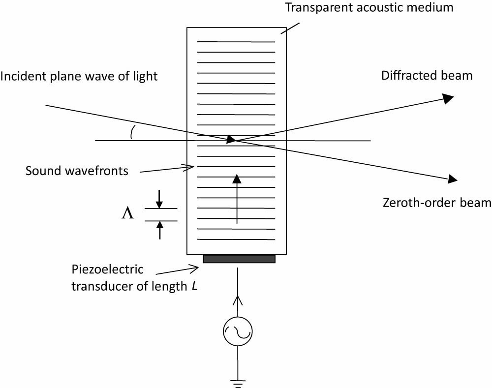
In acousto-optics, we deal with the interaction between sound and light. An AOM consists of a transparent acoustic medium, such as dense glass. A piezoelectric transducer is bonded to the acoustic medium to provide propagating sound waves into it. When a sound wave of wavelength $Λ$ propagates into the acoustic medium, it causes perturbations in the index of refraction, which in turn modulates the laser beam traversing the acoustic medium. Figure 1 shows the physical situation of the interaction between sound and light.

Sign up for Chinese Optics Letters TOC. Get the latest issue of Chinese Optics Letters delivered right to you！Sign up now

$AOM illustrating diffraction of light by sound.$

Figure 1.AOM illustrating diffraction of light by sound.

There are a variety ways to explain the interaction between sound and light. When we consider the interaction of plane waves of light and sound, we assume that the length of the transducer $L$ is being sufficiently wide so as to produce straight wavefronts as a plane wave of sound. Because plane waves have well-defined momenta, we consider the plane-wave interaction of sound and light as a collision of photon and phonon particles. The laws of conservation of energy and momentum are among the most fundamental laws of physics in the process of collision. Denoting the wavevectors of the incident light, diffracted plane waves of light and sound by $k_{0}$ , $k_{+ 1}$ , and $K$ , respectively, and assuming the sound wavefronts are approaching the incident light, the law of conservation of momentum gives us $\tilde{h} k_{+ 1} = \tilde{h} k_{0} + \tilde{h} K,$ (1)where $\tilde{h} = h / 2 π$ , and $h$ is Planck’s constant. Simplifying Eq. (1), we have $k_{+ 1} = k_{0} + K .$ (2)

The corresponding law of conservation of energy gives us (after division by $\tilde{h}$ ) $ω_{+ 1} = ω_{0} + Ω,$ (3)where $ω_{0}$ , $Ω$ , and $ω_{+ 1}$ are the frequencies of the incident light, sound, and diffracted light. Equations (2) and (3) give us the so-called upshifted interaction in acousto-optics. In Fig. 2(a), we show the wavevector interaction diagram, and, in Fig. 2(b), we present the experimental configuration. The experimental configuration illustrates that the zeroth-order diffracted beam is traveling along the same direction as the incident beam, and the $+ 1$ st-order diffracted beam is the beam with frequency upshifted by the sound frequency $Ω$ .

$Upshifted Bragg diffraction: (a) wavevector diagram and (b) experimental configuration. Adapted from Ref. [28].$

Figure 2.Upshifted Bragg diffraction: (a) wavevector diagram and (b) experimental configuration. Adapted from Ref. [28].

The two conservation laws can be employed again to give two equations similar to Eqs. (2) and (3) if we exchange the directions of incident and diffracted light. With the so-called downshifted interaction in acousto-optics and corresponding to Eqs. (2) and (3), we have $k_{- 1} = k_{0} - K,$ (4)and $ω_{- 1} = ω_{0} - Ω,$ (5)respectively. The subscript $- 1$ indicates that the frequency of the diffracted beam is downshifted by the sound frequency $Ω$ . Figures 3(a) and 3(b) illustrate Eqs. (4) and (5), respectively.

$Downshifted Bragg diffraction: (a) wavevector diagram and (b) experimental configuration. Adapted from Ref. [28].$

Figure 3.Downshifted Bragg diffraction: (a) wavevector diagram and (b) experimental configuration. Adapted from Ref. [28].

From Figs. 2(a) and 3(a), we note that the wavevector diagrams are closed for both cases of the interaction. As a result, there can only be one critical incident angle, i.e., the Bragg angle, such that plane waves of sound and light can interact. By inspecting either Fig. 2(a) or 3(a), we find the Bragg angle $ϕ_{B}$ as $\sin ϕ_{B} = \frac{| K |}{2 | k_{0} |} = \frac{K}{2 k_{0}} = \frac{λ_{0}}{2 Λ},$ (6)where $λ_{0}$ is the wavelength of light inside the acoustic medium. However, in practice, sound–light interaction happens even though the direction of incident light is not exactly at the Bragg angle, as we do not have exact plane waves of sound. The sound fields actually spread out with an angle approximately equal to $Λ / L$ as they propagate into the medium. As the width of the transducer decreases, the sound field will act less and less like a single plane wave, and it is more appropriate to consider an angular spectrum of plane waves, providing plane waves of sound for the generation of multiple diffracted light beams. In Fig. 4, we show the situation, where diffraction into higher orders of light happens. We see that $k_{+ 1}$ is generated through the diffraction of $k_{0}$ by $K_{+ 1}$ , $k_{+ 2}$ , the second diffracted order of light is generated through the diffraction of $k_{+ 1}$ by $K_{+ 2}$ , and so on, where $K_{\pm p}$ ( $p = 0, \pm 1, \pm 2, \dots$ ) denotes the various components of the plane-wave spectrum of the sound.

$Multiple diffraction. Adapted from Ref. [28].$

Figure 4.Multiple diffraction. Adapted from Ref. [28].

In addition to the Bragg angle of the AOM, there is another important parameter called the Klein–Cook parameter $Q$ , which is defined as^[28,29] $Q = 2 π L \frac{λ_{0}}{Λ^{2}} .$ (7)

If $Q ≫ 1$ ^[28], the modulator is said to be operated in the Bragg region, i.e., for any sound–light interaction to occur, light must be incident at the Bragg angle, and the AOM is called a Bragg cell. In the ideal Bragg regime, only two diffracted orders exist, and $Q$ would have to be infinity or $L \to \infty$ , giving only a single sound plane wave for the acousto-optic interaction.

3. Korpel–Poon Multiple Plane-Wave Scattering Theory

In the previous section, we used the simple particle approach to describe the necessary conditions for Bragg diffraction to occur. Often, we are interested in knowing how the acousto-optic interaction process affects the amplitude distribution among the different diffracted beams. We shall adopt the Korpel–Poon multiple plane-wave theory to understand this aspect, which is summarized as follows^[28,30]. In Fig. 5, we show a typical 2D rectangular sound column with plane-wave light incidence. The Korpel–Poon equations can be used to describe the interaction between plane waves of sound and light^[28]: $\frac{d ψ_{m} (ξ)}{d ξ} = - j \frac{α}{2} e^{- j \frac{1}{2} Q ξ [\frac{ϕ_{inc}}{ϕ_{B}} + (2 m - 1)]} ψ_{m - 1} (ξ) - j \frac{α}{2} e^{j \frac{1}{2} Q ξ [\frac{ϕ_{inc}}{ϕ_{B}} + (2 m + 1)]} ψ_{m + 1} (ξ),$ (8)where $ψ_{m} (ξ)$ is the complex amplitude of the $m$ th-order diffracted plane wave of light in the direction $ϕ_{m} = ϕ_{inc} + 2 m ϕ_{B}$ . The boundary conditions for Eq. (8) are $ψ_{0} (ξ = 0) = ψ_{inc}$ and $ψ_{m} (ξ = 0) = 0$ for $m \neq 0$ . $ξ = z / L$ is the normalized distance inside the modulator, and $ξ = 1$ signifies the exit plane of the modulator. $ϕ_{inc}$ is the incident angle of the plane wave of amplitude $ψ_{inc}$ . Finally, $α$ is the peak phase delay given by $α = C k_{0} A L / 2,$ (9)where $C$ is the strain-optic coefficient of the acoustic medium, and $A$ is the amplitude of sound, with the sound field given by propagating wave $A \cos (Ω t - K x)$ . Hence, $α$ denotes the strength of the sound amplitude. As a final note, all of the angles are measured from the horizontal axis, and the convention for angles is counterclockwise positive.

Figure 5.AOM modeled by a column of sound of width L. Adapted from Ref. [28].

For a given value of $α$ and $Q$ , the solution to the infinite coupled differential equation in Eq. (8) represents the contributions to the $m$ th-order plane wave of light, $ψ_{m} (ξ = 1)$ , owing to the incident plane wave $ψ_{inc}$ at $ϕ_{inc}$ .

4. Transfer Functions and Acousto-Optic Spatial Filtering

For many decades, the use of acousto-optics has been extensively confined to signal processing. The reason is that AOMs are one-dimensional (1D) devices, and the interaction between light and sound is confined on a plane defined by the wavevectors of sound and light. The use of AOMs operating in the Bragg regime for 2D image processing was pioneered by Xia et al.^[8], and the research is built on the concept of acousto-optic transfer functions first introduced by Poon and Chatterjee^[31]. The concept of transfer functions has also been used for the investigation of beam shaping and beam distortion in thick gratings^[16–18,32].

We consider upshifted Bragg diffraction with off-Bragg angle incidence and limit to two diffracted orders. Hence, we let $ϕ_{inc} = - (1 + δ) ϕ_{B}$ , where $δ$ represents the deviation of the incident plane wave away from the exact Bragg angle. Equation (8) becomes $\frac{d ψ_{0} (ξ)}{d ξ} = - j \frac{α}{2} e^{- j δ Q ξ / 2} ψ_{1} (ξ),$ (10a)and $\frac{d ψ_{1} (ξ)}{d ξ} = - j \frac{α}{2} e^{j δ Q ξ / 2} ψ_{0} (ξ),$ (10b)with the initial conditions $ψ_{0} (ξ = 0) = ψ_{inc}$ , and $ψ_{1} (ξ = 0) = 0.$ Equation (10) can be solved analytically, and the solutions are given by the well-known Phariseau formula^[33]: $ψ_{0} (ξ) = ψ_{inc} e^{- j δ Q ξ / 4} {\cos {[{(δ Q / 4)}^{2} + {(α / 2)}^{2}]}^{1 / 2} ξ + \frac{j δ Q}{4} \frac{\sin {[{(δ Q / 4)}^{2} + {(α / 2)}^{2}]}^{1 / 2} ξ}{{[{(δ Q / 4)}^{2} + {(α / 2)}^{2}]}^{1 / 2}}},$ (11a) $ψ_{1} (ξ) = ψ_{inc} e^{j δ Q ξ / 4} {- j \frac{α}{2} \frac{\sin {[{(δ Q / 4)}^{2} + {(α / 2)}^{2}]}^{1 / 2} ξ}{{[{(δ Q / 4)}^{2} + {(α / 2)}^{2}]}^{1 / 2}}} .$ (11b)

These solutions represent the plane-wave solutions that are due to oblique incidence and have been used for thick hologram gratings^[34]. By letting $δ = 0$ , we can reduce these solutions to the following well-known expressions for exact Bragg incidence: $ψ_{0} (ξ) = ψ_{inc} \cos (\frac{α ξ}{2}),$ (12a)and $ψ_{1} (ξ) = - j ψ_{inc} \sin (\frac{α ξ}{2}) .$ (12b)

Equation (11) motivated Poon and Chatterjee^[15,31] to define the so-called plane-wave transfer function of the AOM. The transfer functions of the zeroth-order beam and the first-order beam are defined, respectively, as follows: $H_{0} (δ) = \frac{{ψ_{0} (ξ) |}_{ξ = 1}}{ψ_{inc}} = e^{- j δ Q / 4} {\cos {[{(δ Q / 4)}^{2} + {(α / 2)}^{2}]}^{1 / 2} + \frac{j δ Q}{4} \frac{\sin {[{(δ Q / 4)}^{2} + {(α / 2)}^{2}]}^{1 / 2}}{{[{(δ Q / 4)}^{2} + {(α / 2)}^{2}]}^{1 / 2}}},$ (13a) $H_{1} (δ) = \frac{{ψ_{1} (ξ) |}_{ξ = 1}}{ψ_{inc}} = e^{j δ Q / 4} {- j \frac{α}{2} \frac{\sin {[{(δ Q / 4)}^{2} + {(α / 2)}^{2}]}^{1 / 2}}{{[{(δ Q / 4)}^{2} + {(α / 2)}^{2}]}^{1 / 2}}} .$ (13b)

These transfer functions show angular selectivity, and they depend on the angle of incidence of the light incident on the AOM. The transfer functions can be written as a function of spatial frequency if we inspect the interaction geometry shown in Fig. 6.

$Diffraction geometry for upshifted Bragg operation. Adapted from Ref. [28].$

Figure 6.Diffraction geometry for upshifted Bragg operation. Adapted from Ref. [28].

$ψ_{inc} (x^{'})$ , $ψ_{0} (x^{'})$ , and $ψ_{1} (x^{''})$ are the incident beam, zeroth-order diffracted beam, and first-order diffracted beam, respectively. For instance, the incident beam can be decomposed into multiple plane waves with different amplitudes propagating in directions defined by $ϕ^{'} = δ \times ϕ_{B}$ . The different amplitudes are simply given by Eq. (13a). Since the spectrum of $ψ_{inc} (x^{'})$ is $F {ψ_{inc} (x^{'})} = Ψ_{inc} (k_{x}^{'}),$ (14)where $k_{x}^{'}$ is the spatial frequency associated with the $x^{'}$ coordinate, we can write $k_{x}^{'} = k_{0} \sin ϕ^{'} \approx k_{0} ϕ^{'} = k_{0} \times δ \times ϕ_{B} = π δ / Λ,$ (15)where we have used the definition of the Bragg angle to arrive at the last step of the equation. With Eq. (15), Eqs. (13a) and (13b) become $H_{0} (k_{x}^{'} Λ / π) = e^{- j k_{x}^{'} Λ Q / 4 π} {\cos {[{(k_{x}^{'} Λ Q / 4 π)}^{2} + {(α / 2)}^{2}]}^{1 / 2} + \frac{j k_{x}^{'} Λ}{4 π} \frac{\sin {[{(k_{x}^{'} Λ Q / 4 π)}^{2} + {(α / 2)}^{2}]}^{1 / 2}}{{[{(k_{x}^{'} Λ Q / 4 π)}^{2} + {(α / 2)}^{2}]}^{1 / 2}}},$ (16a)and $H_{1} (k_{x}^{''} Λ / π) = e^{j k_{x}^{''} Λ Q / 4 π} {- j \frac{α}{2} \frac{\sin {[{(k_{x}^{''} Λ Q / 4 π)}^{2} + {(α / 2)}^{2}]}^{1 / 2}}{{[{(k_{x}^{''} Λ Q / 4 π)}^{2} + {(α / 2)}^{2}]}^{1 / 2}}},$ (16b)where $k_{x}^{''}$ is the spatial frequency associated to the $x^{''}$ coordinate. Now, for example, we can relate the input (incident) spectrum, $Ψ_{inc} (k_{x}^{'})$ , to the spectrum of the zeroth-order beam, $Ψ_{0} (k_{x}^{'})$ , as $Ψ_{0} (k_{x}^{'}) = Ψ_{inc} (k_{x}^{'}) H_{0} (k_{x}^{'} Λ / π),$ and the output beam profile for the zeroth-order diffracted beam is $ψ_{0} (x^{'}) = F^{- 1} {Ψ_{0} (k_{x}^{'})} = F^{- 1} {Ψ_{inc} (k_{x}^{'}) H_{0} (k_{x}^{'} Λ / π)} .$ (17a)

A similar expression exists for the first-order diffracted beam: $ψ_{1} (x^{''}) = F^{- 1} {Ψ_{1} (k_{x}^{''})} = F^{- 1} {Ψ_{inc} (k_{x}^{''}) H_{1} (k_{x}^{''} Λ / π)},$ (17b)where the transfer function of the first-order beam is used. Characteristics of $| H_{0} (k_{x}^{'}) |$ versus $k_{x}^{'}$ and $| H_{1} (k_{x}^{''}) |$ versus $k_{x}^{''}$ for a typical AOM of $Λ = 0.01 mm$ with $Q = 14$ and $Q = 28$ are shown in Fig. 7. The solid lines and the dashed lines are for the cases of $α = 1.0 π$ and $α = 0.65 π$ , respectively. We can clearly observe the programmability of the AOM, as $α$ is proportional to the sound pressure, and $Q$ is a function of the sound frequency as $Q = 2 π L \frac{λ_{0}}{Λ^{2}} = \frac{L λ_{0}}{2 π V_{s}^{2}} Ω^{2}$ , where $V_{s}$ is the sound velocity in the acoustic medium.

Figure 7.Characteristics of |H₀(k_x^′)| and |H₁(k_x^′′)| as a function of Q and α. (a) and (b) Transfer function for the zeroth-order beam and the first-order beam at Λ = 0.01 mm with Q = 14, respectively; (c) and (d) transfer function for the zeroth-order beam and the first-order beam at Λ = 0.01 mm with Q = 28, respectively.

Acousto-optic spatial filtering to the incident beam $ψ_{inc} (x^{'})$ as an input image is computed according to Eq. (17). Indeed, the conversion from a Gaussian laser beam into flattop profiles has been investigated using the transfer function of the first-order beam, which has many important applications such as laser fusion, laser printing, and optical data processing^[15–19,32]. Figure 8 shows an example of flattop profile shaping of a Gaussian laser beam upon Bragg diffraction for the first-order diffracted beam in the far field.

Figure 8.Flaptop beams obtained by the fine tuning of Q or α (alpha) through H₁(k_x^′′Λ/π). Input laser beam is of the profile e^−x²/2σ². Reprinted with permission from Ref. [16] © The Optical Society.

The transfer function of the zeroth-order beam has been used for the investigation of image processing. We place an AOM near the object in an optical imaging setup, as shown in Fig. 9. The object is placed on the input plane, and the output plane is the image plane. The AOM is rotated by the Bragg angle, i.e., $ϕ_{inc} = - ϕ_{B}$ for upshifted interaction configuration. When the AOM is turned off, i.e., $α = 0$ , point A is imaged onto point B. With AOM turned on, the first diffracted order appears, and point B' is formed. In the experiment reported, the size of each of the letter is about $2 mm \times 2 mm$ . The focal length of the lens is 195 mm. $α = 0.65 π$ and $Q = 28$ are used for the AOM.

$Diffraction by AOM and image formation by lens.$

Figure 9.Diffraction by AOM and image formation by lens.

Figure 10 displays the first experimental results using an AOM for image processing.

Figure 10.Experimental results on the output plane: (a) image of the object on the output plane when the AOM is turned off; (b) images of the zeroth-order (left) and the first-order (right) beams. Reprinted from Ref. [8]. Note that the figures presented here are the actual images from the original printed article. The PDF version of the figures provided by the publisher has been smeared.

5. Illustrative Examples

In this section, we illustrate that AOMs can perform some of the optical computing operations such as the important differentiation operations.

5.1. First–order partial derivative

Let us assume that $α / 2 ≫ {(k_{x}^{'})}_{\max} Λ Q / 4 π$ , where ${(k_{x}^{'})}_{\max}$ is the maximum frequency of the input image, so Eq. (16a) becomes $H_{0} (k_{x}^{'} Λ / π) = e^{- \frac{j k_{x}^{'} Λ Q}{4 π}} (A + j B k_{x}^{'}),$ (18)where $A = \cos (\frac{α}{2})$ and $B = \frac{Λ Q}{4 π} \frac{\sin (\frac{α}{2})}{\frac{α}{2}}$ . The exponential term is simply related to the spatial position shift of the diffracted beam along the $x^{'}$ direction, and hence it is inconsequential to image processing. Under this condition, Eq. (18) becomes $H_{0} (k_{x}^{'} Λ / π) \approx A + j B k_{x}^{'} .$ (19)

Assuming the incident beam is of two transverse dimensions, i.e., $ψ_{0} (x^{'}, y^{'}),$ Eq. (17a) now gives $ψ_{0} (x^{'}, y^{'}) = F^{- 1} {Ψ_{inc} (k_{x}^{'}, k_{y}^{'}) H_{0} (k_{x}^{'} Λ / π)} = F^{- 1} {Ψ_{inc} (k_{x}^{'}, k_{y}^{'}) (A + j B k_{x}^{'})} = (A - B \frac{\partial}{\partial x^{'}}) ψ_{inc} (x^{'}, y^{'}) .$ (20)

Note that we can only process the image in one dimension. If we choose the correct value for $α$ , such as $α = π, 3 π, 5 π$ , we can make $A = 0$ . Under this condition, Eq. (20) becomes $ψ_{0} (x^{'}, y^{'}) = - B \frac{\partial ψ_{inc} (x^{'}, y^{'})}{\partial x^{'}},$ (21)which is a pure differentiation operation. For the input image of $4 mm \times 4 mm$ shown in Fig. 11(a), its magnitude spectrum is shown in Fig. 11(b). Figure 11(c) shows the intensity of the first-order light, illustrating the first-order derivative operation. In the simulation, we have taken $α = 3 π$ , $Q = 28$ , and $Λ = 0.1 mm$ for $H_{0} (k_{x}^{'} Λ / π)$ .

Figure 11.(a) Input square object, (b) magnitude spectrum of (a), and (c) intensity of the zeroth-order light.

5.2 Higher–order partial derivative

To obtain higher derivative operations, we can, for example, have two AOMs cascaded. The situation is shown in Fig. 12(a). We use the zeroth-order light output of the first modulator as the input to the second modulator. We then track the zeroth-order light of the second modulator as a final output. Mathematically, the output after the first AOM, from Eq. (20), is $ψ_{0}^{(1)} (x^{'}, y^{'}) = (A_{1} - B_{1} \frac{\partial}{\partial x^{'}}) ψ_{inc} (x^{'}, y^{'}) .$ (22)

Figure 12.(a) Cascaded AOM system and (b) intensity of the zeroth-order light |ψ₀⁽²⁾(x^′, y^′)|² at the exit of the cascade AOM system illustrating second-order differentiation operation.

Similarly, the zeroth-order light after the second AOM is $ψ_{0}^{(2)} (x^{'}, y^{'}) = (A_{2} - B_{2} \frac{\partial}{\partial x^{'}}) ψ_{0}^{(1)} (x^{'}, y^{'}),$ (23)where $A_{1}$ , $B_{1}$ and $A_{2}$ , $B_{2}$ are the same functional forms as $A$ and $B$ , which are the parameters of the first and second AOMs, respectively. By substituting Eq. (22) into Eq. (23), we have $ψ_{0}^{(2)} (x^{'}, y^{'}) = [B_{1} B_{2} \frac{\partial^{2}}{\partial {x^{'}}^{2}} - (A_{1} B_{2} + A_{2} B_{1}) \frac{\partial}{\partial x^{'}} + A_{1} A_{2}] ψ_{inc} (x^{'}, y^{'}) .$ (24)

Note that if $A_{1}$ and $A_{2}$ are designed to be zero, we perform a second-order partial derivative of the incident profile. Figure 12(b) illustrates the result of taking the second-order derivative operation, where the input image is the same as that shown in Fig. 11(a) with parameters $α = 3 π$ , $Q = 28$ , and $Λ = 0.1 mm$ in $H_{0} (k_{x}^{'} Λ / π)$ used for the two AOMs.

5.3 Mixed partial derivative

The acousto-optic interaction is confined to two dimensions, i.e., in the $x z$ plane, as shown in Fig. 6. This limitation restricts its applications to 1D image processing. We can extend the technique to 2D image processing by orienting the second AOM in Fig. 12(a) at an angle with respect to the first AOM. For example, the two AOMs can be aligned orthogonally to each other. If the first AOM is confined in the $x z$ plane with sound propagating along the $x$ direction, the second AOM can be confined in the xy plane with the direction of propagating sound along the $y$ direction. Therefore, the zeroth-order light after the second AOM is given by $ψ_{0}^{(2)} (x^{'}, y^{'}) = (A_{2} - B_{2} \frac{\partial}{\partial y^{'}}) ψ_{0}^{(1)} (x^{'}, y^{'}),$ (25)where $ψ_{0}^{(1)} (x^{'}, y^{'})$ is given by Eq. (22). By substituting Eq. (22) into Eq. (25), we have $ψ_{0}^{(2)} (x^{'}, y^{'}) = (A_{2} - B_{2} \frac{\partial}{\partial y^{'}}) (A_{1} - B_{1} \frac{\partial}{\partial x^{'}}) ψ_{inc} (x^{'}, y^{'}) .$ (26)Again, by choosing $A_{1} = A_{2} = 0$ , we have $ψ_{0}^{(2)} (x^{'}, y^{'}) = B_{1} B_{2} \frac{\partial^{2} ψ_{inc} (x^{'}, y^{'})}{\partial y^{'} \partial x^{'}},$ (27)which accomplishes the mixed partial derivative. Figure 13 shows the intensity light ${| ψ_{0}^{(2)} (x^{'}, y^{'}) |}^{2}$ at the exit of the second AOM for the input profile image of Fig. 11(a). Again, the simulation parameters for the two AOMs are $α = 3 π$ , $Q = 28$ , and $Λ = 0.1 mm$ .

Figure 13.Intensity of the zeroth-order light |ψ₀⁽²⁾(x^′, y^′)|² at the exit of the cascade AOM system.

Depending on applications, the first derivative gives a maximum at the edge location in image processing, and the second derivative gives a zero at the edge location. The mixed derivative provides corner detection commonly used in computer vision to extract certain kinds of features and infer the contents of an image. In addition, corner detection is often used in image registration and image recognition.

6. State-of-the-Art Considerations

In the previous section, we found that the use of AOMs effectively perform a variety of partial derivatives. In this section, we discuss a couple of the latest considerations that would enhance the capability of using AOM(s) for image processing applications.

6.1 AOMs within a Mach–Zehnder interferometer

We consider two AOMs to be used within a Mach–Zehnder interferometer, as shown in Fig. 14. In principle, the two AOMs can be rotated arbitrarily along the xy plane. Irises 1 and 2 are used to select the different diffracted orders for display. The upper arm and the lower arm of the interferometry can perform different processing, depending on the orientation of each of the AOMs in the arm. The shutter has control if we have processing operations by a single arm or by both arms of the interferometer. Beamsplitter BS2 would then sum the contributions from each arm. For example, by aligning one AOM along the $x$ direction on the upper arm of the interferometer and another AOM along the $y$ direction on the lower arm, we accomplish the sum of two first derivative operations: $U (x, y) \propto (\frac{\partial}{\partial x^{'}} + \frac{\partial}{\partial y^{'}}) ψ_{inc} (x^{'}, y^{'}),$ (28)if the zeroth diffracted orders are selected to be summed, where $U (x, y)$ is the total complex field reaching the CCD, as the contribution from each arm performs first-order differentiation operation according to Eq. (21).

Figure 14.Dual AOMs in a Mach–Zehnder interferometer.

Figure 15(a) shows the original input image. With the shutter being on and AOM1 oriented at the angle of 135° in the second quadrant in the xy plane, we see that the first-order differentiation operation is performed along the 135° angle, as shown in Fig. 15(b). At the angle of 45° in the first quadrant, processing is missed. The physical reason is that sound waves propagate along the 135° angle, and hence the 2D image is only processed along this direction. Now, with the operation realized by Eq. (28), where one AOM is along the $x$ direction and the other along the $y$ direction, we have isotropic filtering, and a full circle appears, as shown in Fig. 15(c). The configuration in Fig. 14 is quite general in that we can perform anisotropic edge extraction by blocking off one of the arms of the interferometer or perform isotropic edge extraction if the full interferometer is employed.

Figure 15.(a) Input, (b) image processing by a single AOM, and (c) image processing by dual AOMs in a Mach–Zehnder interferometer realizing the computing operation given by Eq. (28).

6.2 Off-Bragg angle incidence

We consider the angular misalignment of the AOM by letting $ϕ_{inc} = - (1 + δ - Δ δ) ϕ_{B} = - (1 - Δ δ) ϕ_{B} + δ ϕ_{B}$ , where $Δ δ$ represents the amount of deviation from the exact Bragg angle incidence. We call this angular deviation the tilt angle, $Δ δ$ . In other words, when $Δ δ = 0$ , the input image is incident exactly at the Bragg angle. With $ϕ_{inc}$ given above, the zeroth-order transfer function, from Eq. (16a), becomes $H_{0} (\frac{k_{x}^{'} Λ}{π} - Δ δ),$ (29)as $δ$ has been replaced by $δ - Δ δ$ in Eq. (13a). This simply means that the transfer function is shifted from $k_{x}^{'} = 0$ to a new center given by $k_{c}^{'} = \frac{Δ δ π}{Λ} .$ (30)

The highpass characteristic of the zeroth-order transfer function shown in Figs. 7(a) and 7(c) has become a single-sided notch filter with the center frequency given by Eq. (30). The amount of shift depends on the tilt angle. Figure 16(a) shows the image of a 1D chirp grating $t (x, y) = 1 + \cos (100 x^{2})$ , and Fig. 16(b) shows a normalized intensity of the line trace across the red line in Fig. 16(a).

Figure 16.(a) Image of a 1D chirp grating and (b) line trace across the red line in (a).

For $Δ δ = 0.15$ , i.e., the tilt angle is $0.15 ϕ_{B}$ away from the exact Bragg angle incident, Fig. 17(a) shows the spectrum of the chirp grating and the shifted zeroth-order transfer function for $Λ = 0.01 mm$ with $Q = 100$ and $α = π$ . Figure 17(b) shows the processed chirp grating. Note that the part of the image that has been processed shows a dark and blurry area compared to the rest of unprocessed area. Figure 17(c) shows a line trace across the red line of Fig. 17(b).

Figure 17.(a) Spectrum of the chirp grating and shifted zeroth-order transfer function for Δδ = 0.15, (b) processed chirp grating, and (c) line trace across (b).

Figures 18(a) and 18(c) show the processed chirp grating for $Δ δ = 0.2$ and $Δ δ = 0.25$ , respectively, and, in Figs. 18(b) and 18(d), we show the line trace across Figs. 18(a) and 18(c), respectively. In general, by comparing Figs. 17(b), 18(a), and 18(c), we observe that the “dark band” moves to the right of the image as we increase the tilt angle.

Figure 18.Processed images for (a), (b) Δδ = 0.2 and (c), (d) Δδ = 0.25.

While single-sided notch filtering has been previously investigated^[13], it was not without a special consideration to the AOM. With the consideration of off-Bragg angle incidence, we simply need to provide a slight tilt to the AOM. Notch filtering provides the elimination of noise that exists in a narrow band.

7. Concluding Remarks

We have reviewed Bragg processing using AOMs for real-time programmable spatial filtering. In the review, we have discussed the fundamentals of acousto-optics, which is followed by the summary of the multiple plane-wave theory. From the theory, we have discussed the concept of the acousto-optic transfer function, leading to the applications of spatial filtering. We have then given some illustrative examples on how to implement some of the optical computing operations. Finally, we have mentioned a couple of state-of-the-art considerations that would enhance the processing capabilities of Bragg processing. The first consideration is the use of AOMs within a Mach–Zehnder interferometer to perform the summation of two partial differentiation operations. Conceptually, the Mach–Zehnder interferometer system is elegant. However, practical implementation of the idea is quite challenging, as we need to carefully align the two images for summation. In the second consideration, we have looked at the situation when the incident angle is not exactly at the Bragg angle, thereby introducing the tilt angle. The tilt angle gives rise to single-sided notch filtering or half-plane filtering^[35–37], which may well be worth looking into further. The use of incident light beam at twice the Bragg angle is another way to provide single-sided notch filtering^[38].

References

[1] T.-C. Poon, J.-P. Liu. Introduction to Modern Digital Holography with MATLAB(2014).

[2] D. Peri, A. A. Friesem. Image restoration using volume diffraction gratings. Opt. Lett., 3, 124(1978).

[3] S. Case. Fourier processing in the object plane. Opt. Lett., 4, 286(1979).

[4] Y. Yang, X. Liu, Y. Wu, T. Li, F. Fan, H. Huang, S. Wen. Optical edge detection with adjustable resolution based on liquid crystal polarization gratings. Chin. Opt. Lett., 18, 093501(2020).

[5] L. Zhou, X. Huang, Q. Fu, X. Zou, Y. Bai, X. Fu. Fine edge detection in single-pixel imaging. Chin. Opt. Lett., 19, 121101(2021).

[6] V. I. Balakshy. Acousto-optic cell as a filter of spatial frequencies. Radiotekh. Elektron., 29, 1610(1984).

[7] V. I. Balakshy. Acousto-optic visualization of optical wavefronts [Invited]. Appl. Opt., 57, C56(2018).

[8] J. Xia, D. Dunn, T.-C. Poon, P. P. Banerjee. Image edge enhancement by Bragg diffraction. Opt. Commun., 128, 1(1996).

[9] P. P. Banerjee, D. Cao, T.-C. Poon. Basic image-processing operations by use of acousto-optics. Appl. Opt., 36, 3086(1997).

[10] D. Cao, P. P. Banerjee, T.-C. Poon. Image edge enhancement with two cascaded acousto-optic cells with contrapropagating sound. Appl. Opt., 37, 3007(1998).

[11] V. M. Kotov, S. V. Averin, E. V. Kotov. High-frequency acousto-optic light modulation by double propagation of the beam through two Bragg cells. J. Opt. Technol., 86, 129(2019).

[12] V. M. Kotov. Broadband acousto-optic modulation of optical radiation. Acoust. Phys., 65, 369(2019).

[13] P. P. Banerjee, D. Cao, T.-C. Poon. Notch spatial filtering with an acousto-optic modulator. Appl. Opt., 37, 7532(1998).

[14] J. A. Davis, M. D. Norwak. Selective edge enhancement of images with an acousto-optic light modulator. Appl. Opt., 41, 4835(2002).

[15] M. R. Chatterjee, T.-C. Poon, D. N. Sitter. Transfer function formalism for strong acousto-optic Bragg diffraction of light beams with arbitrary profiles. Acustica, 71, 81(1990).

[16] M. McNeill, T.-C. Poon. Gaussian-beam profile shaping by acousto-optic Bragg diffraction. Appl. Opt., 33, 4508(1994).

[17] Y. A. Abdelaziez, P. P. Banerjee, D. R. Evans. Beam shaping by use of hybrid acousto-optics with feedback. Appl. Opt., 44, 3473(2005).

[18] T. Wang, C. Zhang, A. Aleksov, I. Salama, A. Kar. Gaussian beam diffraction by two-dimensional refractive index modulation for high diffraction efficiency and large deflection angle. Opt. Express, 25, 16002(2017).

[19] K. Yushkov, V. A. Molchanov, Y. I. Balakshy, S. N. Mantsevich. Acousto-optic transfer functions as applied to S laser beam shaping. Proc. SPIE, 10744, 107440Q(2018).

[20] V. B. Voloshinov, T. M. Babkina, V. Y. Molchanov. Two-dimensional selection of optical spatial frequencies by acousto-optic methods. Opt. Eng., 41, 1273(2002).

[21] V. I. Balakshy, D. E. Kostyuk. Acousto-optic image processing. Appl. Opt., 48, C24(2009).

[22] K. B. Yushkov, V. Y. Molchanov, P. V. Belousov, A. Y. Abrosimov. Contrast enhancement in microscopy of human thyroid tumors by means of acousto-optic adaptive spatial filtering. J. Biomed. Opt., 21, 016003(2016).

[23] K. B. Yushkov, V. Y. Molchanov. Hyperspectral imaging acousto-optic system with spatial filtering for optical phase visualization. J. Biomed. Opt., 22, 066017(2017).

[24] V. M. Kotov, S. V. Averin, E. K. Kotov, G. N. Shkerdin. Acousto-optic filters based on the superposition of diffraction fields [Invited]. Appl. Opt., 57, C83(2018).

[25] V. M. Kotov, S. V. Averin. Two-dimensional image edge enhancement using two order of Bragg diffraction. Quantum Electron., 50, 305(2020).

[26] V. M. Kotov. Processing 2D images using the Bragg diffraction. J. Commun. Technol. Electron., 65, 1331(2020).

[27] V. M. Kotov. Two-dimensional image edge enhancement using a spatial frequency filter of two-color radiation. Quantum Electron., 51, 348(2021).

[28] T.-C. Poon, T. Kim. Engineering Optics with MATLAB(2018).

[29] W. R. Klein, B. D. Cook. A unified approach to ultrasonic light diffraction. IEEE Trans. Sonics Ultrason., 14, 123(1967).

[30] R. Appel, M. G. Somekh. Series solution for two-frequency Bragg interaction using the Korpel–Poon multiple-scattering model. J. Opt. Soc. Am. A, 10, 466(1993).

[31] T.-C. Poon, M. R. Chatterjee. Transfer function approach to acousto-optic Bragg diffraction of finite optical beams using Fourier integral. International IEEE/Antennas and Propagation Society Symposium and URSI Radio Science Meeting, 1(1988).

[32] A. V. Gorevoy, A. S. Machikhin, G. N. Martynov, V. E. Pozhar. Spatiospectral transformation of noncollimated light beams diffracted by ultrasound in birefringent crystals. Photonics Res., 9, 687(2020).

[33] P. Phariseau. On the diffraction of light by progressive supersonic waves. Proc. Indian Acad. Sci., 44, 165(1956).

[34] H. Kogelnik. Coupled wave theory for thick hologram gratings. Bell Sys. Tech. J., 48, 2909(1969).

[35] S. Lowenthal, Y. Belvaux. Observation of phase objects by optically processed Hilbert transforms. Appl. Phys. Lett., 11, 49(1967).

[36] X. Yang, W. Jia, D. Wu, T.-C. Poon. On the difference between single-and double-sided bandpass filtering of spatial frequencies. Opt. Commun., 384, 71(2017).

[37] Y. Zhang, T.-C. Poon, P. W. M. Tsang, R. Wang, L. Wang. Review on feature extraction for 3-D incoherent image processing using optical scanning holography. IEEE Trans. Industr. Inform., 15, 6146(2019).

[38] T.-C. Poon, A. Korpel. High efficiency acousto-optic diffraction into the second Bragg order. IEEE Ultrasonics Symposium, 751(1983).