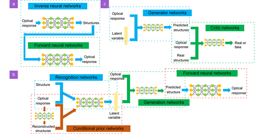
Fig. 1. The structure of three considered models: (a) Tandem networks, (b) VAEs, (c) GANs. The detailed descriptions of building and training each neural networks can be found in the supplementary information.

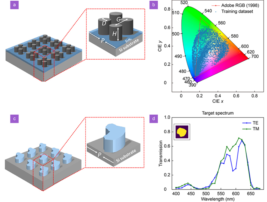
Fig. 2. (a) The template structure for silicon structural color inverse design. Four structural parameters (D, H, G, P) are shown in the inset figure. (b) The obtained structural colors in the training dataset embedded in the CIE 1931 chromatic diagram, which cover a wide color gamut. (c) The free-form structure for silicon transmission filter inverse design. The inset is the period of the structure and the 2D pattern treated as an image. (d) One example of the TE/TM transmission spectra in the training dataset. The inset shows the 2D free-form structure with period 283 nm, where the yellow and black regions are the dielectric material and air, respectively.

Fig. 3. (a) Five randomly selected examples of color inverse design (blue, brown, red, yellow, and green). The first row is the target color, where the inset numbers are the target CIE (x, y, Y) coordinates. The second, third, and forth row corresponds to the predicted structural color by tandem networks, VAE and GAN, respectively, where the inset numbers are the absolute difference of each CIE coordinate. (b) The percent of predicted color tasks that have MAE is smaller than a given threshold. The solid lines show the results when only sampling once for each model, while the dashed lines show results when sampling ten times and picking the most accurate one. As we increase the predicting times, the accuracy of generative models (VAEs and GANs) improved. (c–h) Comparison of one specific application of structural color inverse design: reproducing a paint. (c) The original image of the Vincent van Gogh’s painting: Fishing Boats on the Beach at Saintes Maries-de-la-Mer. (d) The image reconstructed by the predictions of Tandem networks. (e) The image reconstructed by the predictions of the VAE. (f) The image reconstructed by the predictions of VAE when sampling ten times. (g) The image reconstructed by the predictions of GAN. (h) The image reconstructed by the predictions of GAN when sampling ten times. (i–m) The comparison of three models’ robustness with respect to the size of the array for five colors: (i) Blue, (j) Brown, (k) Red, (l) Yellow, (m) Green. To calculate the color, we are not considering the structure to be infinitely periodic anymore. Instead, we are simulating the color within a limited region that only contains the 2 by 2, 3 by 3, 4 by 4, and 5 by 5 array of unit cells, respectively. Fishing Boats on the Beach at Saintes-Maries-de-la-Mer” is reproduced with the permission of the Van Gogh Museum, Amsterdam (Vincent van Gogh Foundation).

Fig. 4. (a) The normalized density distribution of 1000 inverse designed structure parameters for the green color (c) with the CIE coordinates (x, y, Y) = (0.2917, 0.5711, 0.4720). (b) The 3-dimensional color distribution related to 1,000 inverse designed structures. We can see all these predicted structures give a fairly accurate green color. (c) The target green color with coordinates (x, y, Y) = (0.2917, 0.5711, 0.4720). (d) The color corresponding to the structure predicted by tandem networks. (e) The randomly selected 40 different colors corresponding to the structures predicted by the VAE. (f) The randomly selected 40 different colors corresponding to the structures predicted by the GAN.

Fig. 5. Two randomly selected examples of transmission spectrum inverse design for the tandem networks (a)(d), VAEs (b)(e), and GANs (c)(f). The inset shows the original structure (upper) in the test dataset and the inverse predicted structure (lower) by each model.

Fig. 6. Comparisons of the diversity for three models. (a–c) The red bar shows the distribution of the normalized density of irregularity for 1000 inverse predicted structures by tandem networks, VAEs and GANs, while the green points are the scatter plot of spectrum RMSE V.S. the irregularity. According to the distribution of irregularity, we can see that tandem networks only give one structure prediction, where the VAE gives limited diversity, and the GAN gives a multi-modal structure distribution that covers a wide region. (d–f) A randomly chosen inverse designed structure predicted by tandem networks, VAEs and GANs, as well as its corresponding transmission spectra. The inset shows the original structure (upper) in test dataset and the predicted structure (lower) given by each model.

Table 0. Table of performance comparison for the silicon free-form transmission spectrum inverse design. The best results are given by bold type. All MAE, RMSE, and robustness are averaged in three models, which are trained from different random seeds. Their standard deviations are also given.

Table 0. Conclusion of performance measure for all three neural networks. The number of stars is proportional to the performance.

Table 0. Table of performance comparisons for the silicon structure color inverse design problem. Best results are given by bold type. All R² scores, MAE, RMSE, and robustness are averaged in five models, which are trained from different random seeds. Their standard deviations are also given.