Taigao Ma, Mustafa Tobah, Haozhu Wang, L. Jay Guo. Benchmarking deep learning-based models on nanophotonic inverse design problems[J]. Opto-Electronic Science, 2022, 1(1): 210012-1
Copy Citation Text
Photonic inverse design concerns the problem of finding photonic structures with target optical properties. However, traditional methods based on optimization algorithms are time-consuming and computationally expensive. Recently, deep learning-based approaches have been developed to tackle the problem of inverse design efficiently. Although most of these neural network models have demonstrated high accuracy in different inverse design problems, no previous study has examined the potential effects under given constraints in nanomanufacturing. Additionally, the relative strength of different deep learning-based inverse design approaches has not been fully investigated. Here, we benchmark three commonly used deep learning models in inverse design: Tandem networks, Variational Auto-Encoders, and Generative Adversarial Networks. We provide detailed comparisons in terms of their accuracy, diversity, and robustness. We find that tandem networks and Variational Auto-Encoders give the best accuracy, while Generative Adversarial Networks lead to the most diverse predictions. Our findings could serve as a guideline for researchers to select the model that can best suit their design criteria and fabrication considerations. In addition, our code and data are publicly available, which could be used for future inverse design model development and benchmarking.Photonic inverse design concerns the problem of finding photonic structures with target optical properties. However, traditional methods based on optimization algorithms are time-consuming and computationally expensive. Recently, deep learning-based approaches have been developed to tackle the problem of inverse design efficiently. Although most of these neural network models have demonstrated high accuracy in different inverse design problems, no previous study has examined the potential effects under given constraints in nanomanufacturing. Additionally, the relative strength of different deep learning-based inverse design approaches has not been fully investigated. Here, we benchmark three commonly used deep learning models in inverse design: Tandem networks, Variational Auto-Encoders, and Generative Adversarial Networks. We provide detailed comparisons in terms of their accuracy, diversity, and robustness. We find that tandem networks and Variational Auto-Encoders give the best accuracy, while Generative Adversarial Networks lead to the most diverse predictions. Our findings could serve as a guideline for researchers to select the model that can best suit their design criteria and fabrication considerations. In addition, our code and data are publicly available, which could be used for future inverse design model development and benchmarking.
Introduction
Nanophotonics has become an important platform for exploring the light-matter interaction1-5 and wavefront manipulation6-12, and is critical for realizing the advanced photonic-electronic integrated circuits13. Most nanophotonic devices are based on carefully designed nanostructured plasmonic14 and dielectric15 materials. These emerging devices have surpassed conventional photonic devices for many applications, such as on-chip coherent light sources16-17, communication18-19, information processing20, and sensing21-22, to name an important few.
Nanophotonic devices usually have different structures, which can uniquely determine their optical responses and functionality. Researchers can simulate or measure the optical response of a nanophotonic device through the electromagnetic (EM) simulation or experiment. However, it is nontrivial to inverse design the nanostructures from desired optical responses and features. One of the challenges is that different structures can have similar responses, which leads to the one (optical response) -to-many (structures) mapping issue. Usually, inverse design problems are solved by human experts through a time-consuming iterative trial-and-error approach, which is guided by domain knowledge. For example, to realize a polarization-insensitive optical response, the symmetric structure should be typically considered23-24. However, because of the one-to-many mapping issue, we still do not know if the intuitive symmetric structure gives the best performance. Additionally, relying on human expertise alone to design complicated structures with a large number of degrees of freedom (DOF) could result in a slow design process.
On the other hand, optimization-based methods have been widely used in inverse design for a long time25. The optimization-based methods are a combination of forward simulations and automatic iterative searches, where in each iteration, the optimization starts from a set of structures and requires the EM simulations to obtain the corresponding optical responses. The difference between the simulated and the target optical response is later used to update the structures with the objective of minimizing this difference. After sufficient iterations, a structure with desired optical responses can be found. Different optimization methods differ from each other in terms of the mechanism for updating the structure, including the local optimization, e.g., Newton’s methods26 and gradient descent27, and the global optimization, such as simulated annealing28, adjoint variable algorithms29, evolutionary algorithms30, particle-swarm algorithms31, and Bayesian optimization32. A summary and benchmark of optimization methods in the photonic inverse design can be found in ref.33.
Though proven powerful for a wide range of nanophotonic inverse design problems, optimization-based methods are often target-specific, i.e., the optimization process needs to start from scratch for each new inverse design target. Because EM simulation is performed each iteration during the optimization-based inverse design process, applying such methods for many different inverse design targets is time-consuming or even intractable. For example, when designing photonic nanostructures to reconstruct all colors in a painting34, one needs to perform the optimization process for potentially thousands of different inverse design problems, which can take an extremely long time.
Recently, deep learning models have been demonstrated as an efficient alternative to the optimization-based methods for nanophotonic inverse design. Rather than target-specific as in optimization-based methods, deep learning models have a strong generalization ability and can learn the mapping between the structural parameters and the optical responses. After being trained on a dataset containing pairs of structural parameters and the corresponding optical responses, deep learning models can accurately predict the structural parameters given a design target within milliseconds, which greatly improves the efficiency of the inverse design process. For example, Liu et al.35 trained the tandem networks for the inverse design of optical multilayer thin films. Ma et al.36 applied Variational Auto-Encoders (VAEs) for the inverse design of metamaterial elements, including cross, split-ring, and H-shape nanostructures. Liu et al.37 used the Generative Adversarial Networks (GANs) to inverse design the nanostructures for customer-defined optical spectra. There have been several excellent reviews on deep learning-based inverse design published recently, including these three commonly used models for inverse designs38-41.
Although deep learning-based methods have been shown to give accurate predictions efficiently on different nanophotonic inverse design problems, existing works mostly overlook other requirements that are also important for real applications. For example, due to the constraint of existing nanofabrication techniques, structures with high-aspect-ratio or sharp corners can be difficult or even impossible to realize. Therefore, if a diverse set of designs with optical responses close to the target responses can be identified, researchers can choose designs with lower aspect-ratios or smoother shapes that are more amenable to nanofabrication. Thus, whether and to what extent an inverse design method can learn the one-to-many mapping, i.e., come up with a diverse set of designs for a single design target, is a critical feature of practical inverse design methods. Apart from diversity, robustness also plays an important role when considering the real fabrication. If the predicted structures from certain inverse design models violate physical constraints, e.g., the dimension of the designed nanostructure for a metasurface exceeds the size of a unit cell, those structures should never be considered because their optical responses will not be reasonable. In addition, optical responses of fabricated structures may deviate from the desired responses because of the variations in the fabrication process, i.e., the fabrication tolerance. The optical responses corresponding to the predicted structures given by different models may have different sensitivity to such fabrication variations. We believe that in addition to accuracy, both the diversity of the predicted structures and the robustness of their optical response against predicted structures are important considerations when applying deep learning models to inverse design. Unfortunately, no existing work has systematically considered and compared these two properties.
To bridge the gap of the diversity and robustness for deep learning-based inverse design models, and provide a direct comparison for design accuracy, we benchmark three widely used deep learning models: Tandem networks, VAEs, and GANs, on two representative nanophotonic inverse design problems. Performance metrics including accuracy, diversity, and robustness are quantitatively evaluated on both problems with held-out test datasets. Based on our comparisons, we provide recommendations on how to select from these inverse design models based on different requirements and highlight the important future research directions for developing inverse design models that can be adopted more widely for practical nanophotonic inverse design applications.
Methods
Neural networks (NNs) contain multiple layers of neurons that are connected in series. Each neuron takes in one or multiple inputs from the previous layer, sums up all the inputs based on learnable weights, and passes the outputs through a nonlinear activation as the inputs to the next layer. By stacking multiple layers of neurons together, complex information can be processed by these interconnected neurons, enabling NNs to learn the mapping between inputs and outputs. In terms of the inverse design, the inputs are the optical responses, and the outputs are the designs of structures (i.e., structural parameters). However, using the conventional NNs to inverse design directly will give inaccurate results42. Because of the one-to-many mapping issue, there are multiple possible structures for a given target optical response. Minimizing the loss during training (i.e., the difference between the target structure and designed structures, which are usually represented by the Mean Square Error (MSE)) will make it hard for the conventional NNs to converge and lead NNs to output the averaged structures, which usually will not have the desired optical responses. Therefore, special constructions of NNs are required to deal with this one-to-many mapping issue. The following three models are widely known to solve this issue properly and are commonly used in inverse design and, therefore, are examined in this benchmark work. Specifically, tandem networks43 can learn a one-to-one mapping that accurately maps the given optical response to one of the potential structures. Generative models, including VAEs44 and GANs45, leverage the stochastic generation process to directly capture the one-to-many mapping. We classify these three models into two categories based on whether their outputs are deterministic or stochastic (generative models). We use
to denote optical responses and structures, respectively, and
to denote the latent variables or random variables used in VAEs and GANs, respectively. Detailed network constructions and training can be found in the supplementary information.
Deterministic models
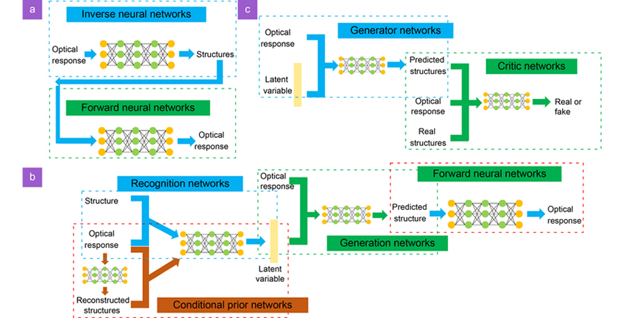
Tandem networks are the combinations of the Forward Neural Networks (FNNs) and the Inverse Neural Networks (INNs), which are shown in Fig. 1(a). The FNN takes in the structure parameters and outputs the predictions of their corresponding optical responses and is used to approximate the solution of Maxwell’s equations. We use the MSE loss to train the FNN:
Figure 1.The structure of three considered models: (a) Tandem networks, (b) VAEs, (c) GANs. The detailed descriptions of building and training each neural networks can be found in the supplementary information.
where
and
are the structures and corresponding optical responses, respectively,
are the predicted responses of FNN based on the network parameters
, and
is the number of training samples. Once trained, we can use the FNN to predict the optical responses accurately for given structures. The INN takes in the target optical responses and outputs inverse predictions of possible structures. The idea of tandem networks is to train the FNN first, and then connect the output of INN to this pre-trained FNN and use the forward prediction loss to supervise the learning of INN:
where
are the predicted structures for given optical responses
based on the INN’s parameters
, and
is the predicted optical responses given by the pre-trained FNN, which correspond to the predicted structures. Using this two-step training, tandem networks circumvent the one-to-many mapping issue by enforcing the INN to converge to only one possible solution suggested by FNN. Tandem networks have been widely used in a variety of inverse design problems, such as multi-layer transmission spectra35, silicon structure colors46, and chiral metamaterials47.
Stochastic models
Unlike tandem neural networks that can only map the input to a single output deterministically, both VAEs and GANs are generative models that can stochastically output multiple different predictions given the same input. For VAEs, we consider a specific variant conditional-VAEs (c-VAEs)44 to inverse predict structures given specific optical responses. There are three networks in VAEs (for the remaining parts, we will use VAEs to refer to c-VAEs for simplicity): the recognition networks, the generation networks, and the conditional prior networks. During training, the recognition networks learn to encode the structures and the optical responses together into the latent variables
, and the generation networks learn to decode the structures from the latent variables
based on the conditional optical responses48. The latent variables
follow the normal distribution. Because of the introduction of latent variables
, VAEs can give multiple predictions when decoding from different latent variables. The conditional prior networks provide reconstructions of structures and are useful during the inverse prediction. We find that connecting the pre-trained FNNs to the output of VAEs can improve the accuracy. The overall network structures for VAEs are shown in Fig. 1(b). The loss for training VAEs is:
where the
is the Kullback-Leibler (KL) divergence between the latent distribution
and prior distribution
,
is the prediction loss between the target structures
and the inverse designed structures
predicted by VAEs,
is the reconstruction loss between the target structures and the reconstructed structures
given by the conditional prior networks,
is the forward prediction loss between the target responses
and the predicted responses given by the FNNs, which correspond to the inverse designed structures
. The
is the weight factor for forward prediction loss. More details can be found in supplementary information.
GANs are another type of generative models. We consider the conditional-GANs (c-GANs)45 to inverse predict structures given specific optical responses. There are two networks in GANs (for remaining parts, we will use GANs to refer to c-GANs for simplicity): the generator networks that generate structures based on the random variables
and the optical responses, and the critic networks that attempt to distinguish if a structure is from the dataset or from the generator networks. The idea of the GAN is based on the game theory, where the generator networks always learn to generate structures that are distributed as close to the test dataset as possible in order to fool the critic networks, while the critic networks always learn to distinguish the generated structures from real structures. The loss for training GANs is:
where
are the predicted structures from the generator networks,
are the scores given by critic networks for the structures from the training dataset, and
are the scores given by critic networks for structures predicted by the generator networks. The
and
are the parameters of the generator and critic networks, respectively. The random variables
are sampled from the normal distribution. We minimize this loss function when training the generator networks, while maximizing this loss function when training the critic networks.
Both VAEs and GANs are widely used in inverse designing free-form structures, including metamaterials36, diffractive metagratings49, and nano-antennas50. Detailed descriptions for constructing and training each model can be found in the supplementary information.
Experiments
We formally introduce two inverse design problems as the benchmarking problems to evaluate inverse design models. A set of evaluation metrics regarding the design accuracy, diversity, and robustness to fabrication variations are later described in detail. We report the benchmarking results and summarize the relative performance of tandem networks, VAEs, and GANs at the end of this section. All data and code are publicly available51.
Inverse design problems
Nanophotonic inverse design problems can be grouped into two categories40 based on the number of DOF associated with the structure design. On the one hand, when the number of DOF is small, a structure template based on simple building block elements, such as nanodisks and nanobricks, can be used to form the design. A few structural parameters, including height, width, and radius, can be carefully designed to describe the structural elements. Thus, a 1D vector containing the structural parameters is used as the representation for the design. On the other hand, when the number of DOF is large, the nanostructures have free-form geometries and cannot be represented by a small set of structural parameters. Instead, 2D binarized images are used to represent these free-form structures. In terms of the construction of neural networks, we use Multilayer Perceptron52 (MLP) and Convolutional Neural Networks53 (CNN) for the vector representation and the image representation, respectively.
To ensure conclusions are generalizable on most nanophotonic inverse design problems, we consider two different inverse design problems from the template design and free-form design categories, respectively.
Template structures: Silicon structure color inverse design
For the inverse design based on template structures, we choose a design task that has been investigated in ref.46. As shown in Fig. 2(a), the template structure is a unit cell arranged periodically and consists of four identical and uniformly spaced silicon nanorods. A layer of 70 nm Si3N4 is located between the nanorod structures and the bottom silicon substrate layer. This periodic template structure is represented by a vector with four structural parameters
, where D and H refer to the diameter and height of each nanorod, respectively,
refers to the gap between two nearby nanorods, and P refers to the period of the unit cell. The inverse design target of optical responses is the reflective structural color, which can be described by three-dimension CIE 1931 coordinates
.
Figure 2.(a) The template structure for silicon structural color inverse design. Four structural parameters (D, H, G, P) are shown in the inset figure. (b) The obtained structural colors in the training dataset embedded in the CIE 1931 chromatic diagram, which cover a wide color gamut. (c) The free-form structure for silicon transmission filter inverse design. The inset is the period of the structure and the 2D pattern treated as an image. (d) One example of the TE/TM transmission spectra in the training dataset. The inset shows the 2D free-form structure with period 283 nm, where the yellow and black regions are the dielectric material and air, respectively.
For data collection, we use the Rigorous Coupled Wave Analysis (RCWA)54 to simulate 8411 samples. Structure parameters of
are uniformly and randomly sampled in the ranges of (80, 160) nm, (30, 200) nm, (160, 320) nm, and (300, 700) nm, respectively. A physical constraint
is used during the sampling process to make sure all four nanorods are within one unit cell. The reflection spectrum is computed between the (380, 780) nm wavelength range with a 5 nm step size, which is then converted to CIE 1931 coordinates
. Detailed information can be found in ref.46. In all three models, we use 6,000 samples for training, 1,000 samples for validation, and the rest 1,411 samples for testing. The obtained structural colors in the training dataset are plotted in the CIE chromatic diagram in Fig. 2(b).
For the inverse design based on free-form structures, we choose a design task that we investigated before, where we used NNs to inverse design metasurface filters55. As shown in Fig. 2(c), the structure is a 2D periodic pattern on the silicon substrate. The pattern is made of polycrystalline silicon (Poly-Si) with a fixed thickness of 500 nm and is represented by a 2D
pixeled binarized image. We also include a scalar parameter ranging from 200 nm to 400 nm as the period of the unit cell. For the inverse design target of optical responses, we consider the transmission spectra for both TE and TM polarized normal incident light. The spectrum target is within the visible band and ranges from 400 nm to 680 nm, with a 10 nm step size.
Again, we use RCWA to simulate 63,757 samples. The free-form 2D patterns are randomly generated, and the period is uniformly and randomly sampled between (200, 400) nm. During the image pattern generation, to make sure the corresponding structures satisfy the fabrication limitation, all sharp features are smoothed to fulfil the minimum curvature with a 20 nm radius. Detailed descriptions can be found in the supplementary information. In all three models, we use 53,750 samples for training, 5000 samples for validation, and 5007 samples for testing. Figure 2(d) gives one example of the free-form structure as well as the corresponding transmission spectra.
Evaluation metrics
As stated earlier, practical inverse design problems often involve considerations beyond accuracy. However, no previous research work has systematically studied the properties of deep learning-based inverse design models for practical applications. To bridge this gap, we propose a set of evaluation metrics based on practical considerations that are generalizable for extensive inverse design problems:
Accuracy: The design accuracy is most widely considered in previous research works, and it quantifies how close we can design a structure that achieves the target response. We use both MAE and Root Mean Square Error (RMSE) to measure the accuracy. The MAE is expressed as:
where
and
refer to the target optical responses and inverse designed optical response, respectively. The RMSE is expressed as:
RMSE is more sensitive to large difference than MAE because of the squared error. Thus, if a design method can output accurate designs on average but predicts poor designs occasionally, its MAE will be low while the RMSE could be high. Therefore, including MAE and RMSE for the accuracy evaluation allows us to investigate if an inverse design model exhibits such behavior.
Diversity: This evaluates if the examined model can give multiple predictions for one specific task; and if so, how diverse these predicted structures are distributed in the structure space. As mentioned above, an inverse design model that can output a diverse set of structure designs given a design target is highly desired. This is because the diverse designs could facilitate the fabrication process by providing more candidate designs for researchers to choose from, which can be beneficial, especially when the designs involve shapes that are challenging for nanofabrication. In addition, an inverse design model that can capture the one-to-many mapping may provide physical insights for the inverse design problems.
Robustness: Two different aspects of robustness are considered. First, we examine the robustness of neural network models by checking if the predicted structures satisfy the constraint of the physical system. In addition, we also examine the optical performance drop caused by fabrication variations as the second type of robustness. This is because during nanofabrication, the fabricated structures may slightly deviate from the expected designs due to variations in the fabrication process, leading to different optical responses.
To compare the performance, we report each model’s best performance on these two inverse design problems found through an extensive hyperparameter search (details in the supplementary information).
Performance comparisons
Template structure: Silicon structure color inverse design
For the aspect of accuracy, we compare the predicted colors given by the inverse designed structures with the target colors. To calculate the predicted colors, we first use RCWA to simulate the reflection spectra for the inverse-designed structures, then covert the spectra into the CIE color coordinates. When measuring the accuracy, in addition to the MAE and RMSE, we also calculate the
scores for each CIE coordinate
. In order to improve the statistics confidence, we train each model five times with five different random seeds. All five models use the same hyperparameters, which are found through the hyperparameters search. We report the average accuracy results of all five models in Table 1, where the standard deviations are also included. More details can be found in the supplementary information. To visualize the difference between the designed color and the target color, we randomly select and show five examples of structural color inverse design given by tandem networks, VAEs, and GANs in Fig. 3(a). Additional results on the color pixel generation to reproduce a painting with the inverse designed structures are also included in Fig. 3(c–h). Based on the high
scores and small MAE and RMSE values, as well as the accurate color inverse predictions, we can see that all these three models can give accurate results of color inverse design, although tandem networks give slightly more accurate results than the VAE and the GAN.
Table Infomation Is Not Enable
Figure 3.(a) Five randomly selected examples of color inverse design (blue, brown, red, yellow, and green). The first row is the target color, where the inset numbers are the target CIE (x, y, Y) coordinates. The second, third, and forth row corresponds to the predicted structural color by tandem networks, VAE and GAN, respectively, where the inset numbers are the absolute difference of each CIE coordinate. (b) The percent of predicted color tasks that have MAE is smaller than a given threshold. The solid lines show the results when only sampling once for each model, while the dashed lines show results when sampling ten times and picking the most accurate one. As we increase the predicting times, the accuracy of generative models (VAEs and GANs) improved. (c–h) Comparison of one specific application of structural color inverse design: reproducing a paint. (c) The original image of the Vincent van Gogh’s painting: Fishing Boats on the Beach at Saintes Maries-de-la-Mer. (d) The image reconstructed by the predictions of Tandem networks. (e) The image reconstructed by the predictions of the VAE. (f) The image reconstructed by the predictions of VAE when sampling ten times. (g) The image reconstructed by the predictions of GAN. (h) The image reconstructed by the predictions of GAN when sampling ten times. (i–m) The comparison of three models’ robustness with respect to the size of the array for five colors: (i) Blue, (j) Brown, (k) Red, (l) Yellow, (m) Green. To calculate the color, we are not considering the structure to be infinitely periodic anymore. Instead, we are simulating the color within a limited region that only contains the 2 by 2, 3 by 3, 4 by 4, and 5 by 5 array of unit cells, respectively. Fishing Boats on the Beach at Saintes-Maries-de-la-Mer” is reproduced with the permission of the Van Gogh Museum, Amsterdam (Vincent van Gogh Foundation).
However, tandem networks can only give one prediction for a specific color task, which could lead to a potential negative impact on fabrication (will be discussed later). Since the VAEs and GANs introduce extra latent variables or random variables, every time they will give different structure predictions44, 45. By inverse predicting the same color task multiple times and choosing the best structure that gives the most accurate color, the accuracy of inverse design for VAEs and GANs can be further improved. In Fig. 3(b), we calculate how many color inverse design tasks have MAE smaller than a specific MAE threshold and show the tendency as the sampling times of inverse prediction change from once to ten times. We can see that when prediction is carried out for ten sampling times, the accuracy of the GAN and VAE is improved, giving a higher percent of tasks for a specific MAE threshold. The accuracy of GAN is improved more than the improvement of VAE, which is related to the diversity of each neural network and will be discussed later. In addition, we do want to mention that inverse predicting multiple times costs extra time since it requires more simulations for validating the predicted colors and picking up the best structure.
For the diversity of the generated candidate structures, we compare how diverse the distributions of the predicted structures are for each neural network model. Specifically, we start from the inverse design of the green color with the CIE coordinates
. The original green color is shown in Fig. 4(c). For each model, we inverse predict 1000 times using this specific color target as the input, which gives 1000 predicted structures. To visualize and compare the distribution, we first calculate the frequency histogram of each predicted structure parameter, then divide each histogram by its respective maximum value to ensure that the peak density for each histogram is one. We show this normalized density of each structure parameter
in Fig. 4(a). Since the tandem networks are deterministic models, these 1,000 predicted structures are the same, i.e., there is no diversity at all. Both VAEs and GANs can give diverse structure distributions, but with different levels of diversity. For the VAEs, since the recognition networks learn to map structures into a single-modal normal distribution, they can only output a narrow and single-peaked structural distribution. In comparison, there is no such limitation for GANs, therefore, they can capture a multi-modal distribution caused by the intrinsic one-to-many mapping, where the learned structure distributions of height, period, and diameter exhibit multiple peaks. The overlapped distributions of structural parameters show that both the tandem networks and the VAEs methods only learn one specific mode in the multi-modal distribution learned by GANs. This diverse distribution in structure space clearly reveals the intrinsic one-to-many mapping feature, which is expected in physics.
Figure 4.(a) The normalized density distribution of 1000 inverse designed structure parameters for the green color (c) with the CIE coordinates (x, y, Y) = (0.2917, 0.5711, 0.4720). (b) The 3-dimensional color distribution related to 1,000 inverse designed structures. We can see all these predicted structures give a fairly accurate green color. (c) The target green color with coordinates (x, y, Y) = (0.2917, 0.5711, 0.4720). (d) The color corresponding to the structure predicted by tandem networks. (e) The randomly selected 40 different colors corresponding to the structures predicted by the VAE. (f) The randomly selected 40 different colors corresponding to the structures predicted by the GAN.
To validate the color accuracy of 1000 predicted structures in such diverse distributions, we simulate the colors of these structures using RCWA and show all predicted colors in the 3d
space in Fig. 4(b). For further comparison, we randomly show 40 colors predicted by the VAE and GAN in Fig. 4(e, f). The color predicted by the tandem networks is also shown in Fig. 4(d). Although the predicted structures are broadly distributed, their corresponding colors are close to the target color (an illustration of the one-to-many mapping), and their color differences cannot be distinguished by human eyes. This diverse distribution is highly desirable in practice since more broadly distributed structure spaces provide more choices during fabrication. Specifically, structures with greater gaps or greater diameters are easier to fabricate, allowing researchers to pick the structures that are more suitable for fabrication from these 1000 predicted structures. Therefore, when diversity is of high design priority, the GAN will be more preferred in inverse design. More examples with yellow and brown colors can be found in supplementary information, and both give similar conclusions.
We want to emphasize the relationship between accuracy and diversity. In Fig. 4(b), each neural network model exhibits different distribution behaviors in the color space, which originates from the different distributions behaviors in the structure spaces. Tandem networks only give one predicted color that is close to the target color. The colors given by the VAE are located within a narrow color space close to the target color, while the GAN’s are more diversely spread out in the color space, surrounding the target color. Therefore, if we only predict once for the GAN, it is possible that the inverse designed structure gives the color with a large color difference from the target color. By predicting multiple times and picking the most accurate one, we can minimize this randomness and improve the accuracy of the GAN. Similar procedures are also applicable to the VAE, but its accuracy may not be improved too much because the structure distributions are localized, leading to the localized color distribution.
In terms of robustness, there are three aspects to examine. First, we examine if the generated structures satisfy the constraints of physical systems. We need to make sure that all predicted structure parameters are positive and satisfy another physical constraint of
, meaning that the sum of the gap and the diameter of nanorods should be smaller than the period of the unit cell. Any structure that does not satisfy these two constraints is treated as a faultydesign. For a given color design target, we run each model ten times, which gives ten predicted structures. When all ten structures are faultydesigns, this design task is treated as a faultedtask. We calculate the number of faulttasks in the test dataset and summarize the faultrate for each model in Table 1. Another example of analyzing the robustness of the image reconstruction in Fig. 3(c–h) is shown in
Fig. S10. We can see that the chance that tandem networks fail to give a prediction is higher than VAEs and GANs, which could limit its applications when these failed tasks are necessary. Secondly, we examine how generated structures are susceptible to fabrication variations. This is done by adding a +5/–5 nm perturbation to structure parameters and measuring the shifts of CIE coordinates. We randomly select and inverse predict 100 color targets in the test dataset and calculate the color related to the perturbated structures. We use the MAE between this perturbated color and the target color to represent the fabrication robustness, i.e., smaller MAE corresponds to higher robustness. Again, we average the robustness from five different models and show the results in the last column in Table 1. We can see VAE gives slightly higher robustness than the other two models. But overall, all these three models give similar robustness in terms of the fabrication variation. This result aligns with our expectation because the loss functions of all three inverse design models do not include components that promote robustness with respect to fabrication variation.
All of the colors in the training dataset are obtained based on the infinite periodic array of unit cells, which cannot be used in many actual applications, e.g., reproduce a paint. Therefore, we evaluate the third robustness, which is to examine how accurate the predicted colors are when only a finite size of the array of the unit cell are used for one color pixel34. Here we consider that a color pixel is made up of an array with a finite number of unit cells, with array size to be 2 by 2, 3 by 3, 4 by 4, and 5 by 5. Specifically, we calculate and compare the robustness of these five colors in Fig. 3(a) as an example. For each color task, we inverse predict twenty times and choose the best structure that gives the most accurate color. In order to calculate the predicted color related to different sizes of the array of unit cells, because the considered simulation region is no longer periodic, we change the periodic boundary conditions to perfect matching layers and use the Finite-Difference Time-Domain (FDTD) to simulate the reflection spectrum. Detailed descriptions can be found in the supplementary information. We calculate the MAE between the predicted color and target color and show the relationship with respect to the size of the unit cell array in Fig. 3(i–m). As we expected, when we increase the size of the unit cells array, the color difference with respect to the target color decreases. Overall, again generative models, including both VAEs and GANs, are more robust than tandem networks when using a finite array size to reconstruct one color pixel. This is because generative models can give multiple structure predictions, which is possible to provide more robust structures.
In terms of accuracy, we compare the MAE and RMSE between the simulated spectra related to the inverse designed structures and the target spectra. Because the pixel values of predicted 2D image patterns are not exactly zero or one, we binarize the predicted image patterns by setting the binarization threshold to be 0.5. The corresponding transmission spectra are simulated using RCWA based on the binarized 2D image pattens. Again, in order to improve the statistics confidence, we train each model three times with three different random seeds. All three models use the same hyperparameters, which are found through the hyperparameters search. We report the average accuracy results over all three models in Table 2, where the standard deviations are also included. Figure 5 also gives two examples for transmission spectrum inverse design, where the inset (lower) shows the inverse designed 2D structure pattern. By comparison, we can see that if researchers care more about the accuracy, they can refer to tandem networks or VAEs.
Table Infomation Is Not Enable
Figure 5.Two randomly selected examples of transmission spectrum inverse design for the tandem networks (a)(d), VAEs (b)(e), and GANs (c)(f). The inset shows the original structure (upper) in the test dataset and the inverse predicted structure (lower) by each model.
In terms of the diversity, we compare how diverse the distributions of the predicted 2D patterns are for each model. To quantify the diversity of free-form structures, we introduce a quantity to describe the irregularity of 2D patterns, which is defined as:
where
is the distance between the extracted edges and the center of the 2D pattern. We give several examples of the 2D image patterns with different
in the supplementary information.
means a perfect circle pattern and a greater
means a more nonuniform pattern. By examining the distribution of
, we can reveal the distribution of the predicted structures. Some other evaluation methods for irregularity can also be used.
As an example, we start from the inverse design of a randomly chosen target spectrum in Fig. 6. Similarly, for each model, we inverse predict 1000 times using this specific spectrum target as the input, which gives 1,000 predicted structures. We show the normalized density of irregularity distribution in Fig. 6(a–c). Again, we observe that tandem networks only give one structure prediction, while the VAE tends to give a single-peak distribution, and the GAN gives a multi-modal distribution. To better demonstrate that these predicted structures give accurate spectra, we simulate their transmission spectra using the RCWA. In Fig. 6(a–c), we show the MAE of the 1,000 spectra v.s. the irregularity of 1,000 predicted structures. One specific example of the inverse designed structure as well as its transmission spectra is also shown in Fig. 6(d–f). We can see that although the predicted structures are distributed in a wide irregularity range, their spectra are close to the target spectrum. In this case, a more diverse set of structure predictions can benefit the fabrication since a smaller irregularity means a more uniform shape, which leads to easier fabrication. Therefore, researchers can always pick the best structure that can facilitate the fabrication while still giving an accurate spectrum. In this case, the GAN would be more preferred. Another example of diversity in the spectrum inverse design can be found in the supplementary information, which gives similar conclusions.
Figure 6.Comparisons of the diversity for three models. (a–c) The red bar shows the distribution of the normalized density of irregularity for 1000 inverse predicted structures by tandem networks, VAEs and GANs, while the green points are the scatter plot of spectrum RMSE V.S. the irregularity. According to the distribution of irregularity, we can see that tandem networks only give one structure prediction, where the VAE gives limited diversity, and the GAN gives a multi-modal structure distribution that covers a wide region. (d–f) A randomly chosen inverse designed structure predicted by tandem networks, VAEs and GANs, as well as its corresponding transmission spectra. The inset shows the original structure (upper) in test dataset and the predicted structure (lower) given by each model.
In terms of robustness, we only investigate the robustness against fabrication variation, since all generated patterns are images, and they do not need to satisfy any physical constraint similar to the color inverse design task (any negative image pixel can be attributed as 0 during binarization). We measure the fabrication robustness by testing how much the spectrum will shift under a small perturbation of the inverse designed structures, mimicking the fabrication variations induced by nanofabrication tolerance. This is done by shrinking, expanding, or smoothing the shapes of predicted structures by a small factor. More details can be found in the supplementary information. We randomly pick 100 spectrum targets from the test dataset and use the MAE of the perturbated spectra with respect to the target spectra to represent the fabrication robustness. Again, we average the robustness from three different models and show the results in the last column in Table 2. We can see that VAE gives slightly higher robustness than the other two models. But overall, all these three models give similar robustness measurements, which aligns with the observation in the template structure inverse design task.
Results and discussion
For all evaluating metrics including accuracy, diversity, and robustness, we give a qualitative comparison of all three models in Table 3, where a greater number of stars correspond to a better performance in each evaluation metric. We find that tandem networks and VAEs give higher accuracy than GANs. However, tandem networks can fail when predicting some tasks, which can be problematic if this specific task is important because there is no way to find another structure to replace this failed structure. Generative models like VAEs and GANs can solve this problem and give multiple predictions by introducing random variables. GANs give a better diversity than the tandem networks and VAE as well as demonstrate multi-modal outputs for the inverse-designed structures, providing designers with more options to select the best structure. By running predictions multiple times, it is possible to find structures that give more accurate results, thus increasing the accuracy of the GAN. We do not observe a significant difference in robustness among the three studied models, but VAEs give a slightly better result. We need to emphasize that during training, there is no loss function terms or training data that incorporates the fabrication variations. Therefore, the observation that all three models perform similarly in terms of robustness is not surprising.
Although we only consider two specific inverse design problems, these neural networks models and introduced evaluation metrics are applicable for many other nanophotonic inverse design problems with different structures and materials, including the multilayer thin films35, plasmonic nanostructures56, and metasurfaces37, etc, where their structures can be described either by a vector or an image when processed by appropriate neural networks. Therefore, our conclusions are generalizable to a wide range of nanophotonic inverse design problems.
Table Infomation Is Not Enable
Conclusions
In conclusion, we benchmark the performance of three deep learning-based methods that are commonly used in the current deep learning-based inverse design: tandem networks, VAEs, and GANs. To compare their performance and give guidance to researchers and engineers, each model is evaluated in terms of accuracy, diversity, and robustness, where the last two aspects are seldomly explored in the current domain of deep learning-based inverse design. Detailed comparisons and discussions are included. We hope our work can provide insights for researchers and engineers to correctly select their target model that best fits their specific needs. For example, if researchers want the predicted structures to give the most accurate optical responses, then they can choose tandem networks or VAEs. If they want to have multiple structures for easier fabrication, GANs or VAEs will be preferred.
All three models show similar performance on robustness, although VAEs give slightly better performance. Fabrication robustness is very important for real application and should be considered when dealing with nano-fabrications. Additional model development beyond these studied models is necessary to incorporate fabrication robustness as a learning objective. For example, by re-parametrizing the structures57, or building suitable datasets and incorporating the fabrication variation into loss functions58, it is possible for neural networks to learn these properties and output predicted structures that are robust to fabrication variations.
We also want to mention that the current machine learning models can only work well for in-distribution inverse design, where the target optical responses should follow a similar distribution of the training dataset. Otherwise, the NNs may give erroneous predictions. This is because NNs can only accurately interpolate within the training dataset, while the extrapolation capability beyond the training distribution is limited. For inverse design problems that may require a high degree of extrapolation, forward search approaches based on reinforcement learning59 or conventional optimization-based methods should be used. Hybrid methods that combine neural networks with physics-driven solvers can also be used for solving the extrapolation issue60, 61.
We are grateful for financial support from NSF Data Science Supplement of SNM program (CMMI-1635636)
The authors declare no competing financial interests.
Taigao Ma, Mustafa Tobah, Haozhu Wang, L. Jay Guo. Benchmarking deep learning-based models on nanophotonic inverse design problems[J]. Opto-Electronic Science, 2022, 1(1): 210012-1