Target Scale Adaptive Robust Tracking Based on Fusion of Multilayer Convolutional Features

Xin Wang; Zhiqiang Hou; Wangsheng Yu; Zefenfen Jin; Xianxiang Qin

doi:10.3788/AOS201737.1115005

Journals >Acta Optica Sinica >Volume 37 >Issue 11 >Page 1115005 > Article

Acta Optica Sinica
Vol. 37, Issue 11, 1115005 (2017)

Target Scale Adaptive Robust Tracking Based on Fusion of Multilayer Convolutional Features

Xin Wang^*, Zhiqiang Hou, Wangsheng Yu, Zefenfen Jin, and Xianxiang Qin

Author Affiliations

Information and Navigation College, Air Force Engineering University, Xi'an, Shaanxi 710077, China

show less

DOI: 10.3788/AOS201737.1115005 Cite this Article Set citation alerts

Xin Wang, Zhiqiang Hou, Wangsheng Yu, Zefenfen Jin, Xianxiang Qin. Target Scale Adaptive Robust Tracking Based on Fusion of Multilayer Convolutional Features[J]. Acta Optica Sinica, 2017, 37(11): 1115005 Copy Citation Text

show less

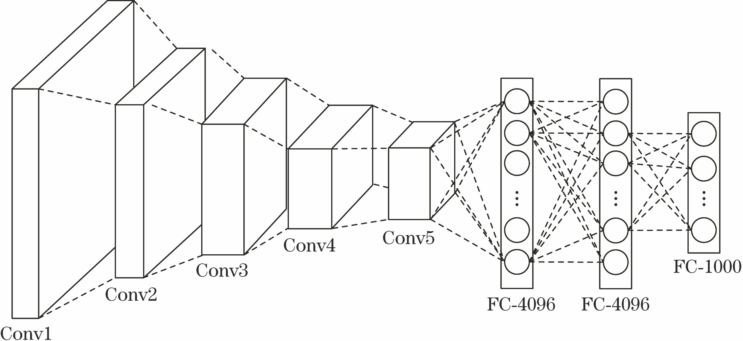
Fig. 1. Schematic of deep convolution network of VGG-Net-19

Download full size

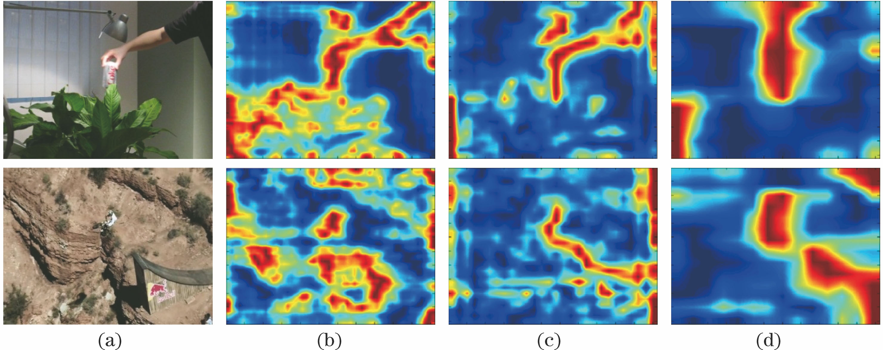
Fig. 2. Visualizations for different convolutional layers of VGG-Net-19. (a) Input images; (b) Conv3-4; (c) Conv4-4; (d) Conv5-4

Download full size

Fig. 3. Construct the scale pyramid of the target by multi-scale sampling

Download full size

Fig. 4. Flow chart of proposed algorithm

Download full size

Fig. 5. Comparison of partial tracking results of seven trackers

Download full size

Fig. 6. Center location error curves of eight test sequences

Download full size

Fig. 7. Overlap rate curves of eight test sequences

Download full size

Fig. 8. (a) Success rate curves and (b) precision curves of 28 test sequences

Download full size

Fig. 9. Tracking performance analysis in different combinations of feature. (a) Success rate curves; (b) precision curves

Download full size

Input: Image sequence: I₁, I₂, …, I_n. Initial target position: p₀=(x₀, y₀), and initial target scale: s₀=(w₀, h₀).
Output: The estimated position of target: p_t=(x_t, y_t), and estimated scale: s_t=(w_t, h_t).
For t=1,2,…,n, do:
1	Locate the Center of Target
1.1	Crop out the ROI image in frame #t centered at p_t_-1, and extract the hierarchical convolutional features;
1.2	Learn the correlation response map using Eq. (5) and Eq. (7) for each convolutional layer;
1.3	Fuse the multiple correlation response maps using Eq. (8), and obtain the compositive response map;
1.4	Locate the center of the target p_t in frame #t using Eq. (9).
2	Estimate the Scale of Target
2.1	Obtain the multi-scale sample images I_s={I_s₁,…, I_sm} in frame #t based on p_t and s_t_-1;
2.2	Build scale filters by extracting HOG features from the above multi-scale sample images;
2.3	Compute the correlation response score using Eq. (10) and Eq. (11);
2.4	Estimate the optimal scale s_t of the target in frame #t using Eq. (12).
3	Model Update
3.1	Update the position filters using Eq. (13);
3.2	Update the scale filters using Eq. (14).
Until End of the image sequence.

Table 1. Scale adaptive robust tracker based on fusion of multilayer convolutional features

Algorithm	SV(28)	IV(15)	OCC(16)	BC(11)	DEF(9)	MB(8)	FM(12)	IPR(18)	OPR(23)	OV(4)	LR(3)
Proposed	0.880	0.838	$\begin{matrix} \bar{0.841} \end{matrix}$	$\begin{matrix} \bar{0.861} \end{matrix}$	0.932	0.870	0.772	0.879	$\begin{matrix} \bar{0.855} \end{matrix}$	0.702	0.873
HCF	0.880	0.858	0.847	0.867	$\begin{matrix} \bar{0.927} \end{matrix}$	$\begin{matrix} \bar{0.844} \end{matrix}$	$\begin{matrix} \bar{0.757} \end{matrix}$	$\begin{matrix} \bar{0.873} \end{matrix}$	0.857	0.656	$\begin{matrix} \bar{0.863} \end{matrix}$
FCNT	$\begin{matrix} \bar{0.830} \end{matrix}$	0.779	0.737	0.713	0.925	0.740	0.715	0.774	0.798	$\begin{matrix} \bar{0.691} \end{matrix}$	0.686
CNN-SVM	0.827	0.751	0.733	0.689	0.890	0.725	0.685	0.793	0.800	0.650	0.606
CNT	0.662	0.521	0.667	0.463	0.686	0.479	0.477	0.583	0.630	0.481	0.410
DSST	0.740	0.681	0.785	0.610	0.733	0.635	0.539	0.714	0.725	0.453	0.402
KCF	0.680	0.632	0.744	0.578	0.734	0.679	0.586	0.619	0.678	0.639	0.233

Table 2. Comparison of the tracking precisions of the algorithm of different attributes

Algorithm	SV(28)	IV(15)	OCC(16)	BC(11)	DEF(9)	MB(8)	FM(12)	IPR(18)	OPR(23)	OV(4)	LR(3)
Proposed	0.600	0.556	0.582	0.586	0.629	$\begin{matrix} \bar{0.591} \end{matrix}$	0.554	0.591	0.579	0.527	0.574
HCF	0.531	0.509	0.514	$\begin{matrix} \bar{0.573} \end{matrix}$	0.589	0.594	$\begin{matrix} \bar{0.545} \end{matrix}$	$\begin{matrix} \bar{0.532} \end{matrix}$	0.525	0.522	$\begin{matrix} \bar{0.497} \end{matrix}$
FCNT	$\begin{matrix} \bar{0.558} \end{matrix}$	$\begin{matrix} \bar{0.551} \end{matrix}$	$\begin{matrix} \bar{0.517} \end{matrix}$	0.506	$\begin{matrix} \bar{0.628} \end{matrix}$	0.552	0.533	0.504	$\begin{matrix} \bar{0.539} \end{matrix}$	0.573	0.451
CNN-SVM	0.513	0.477	0.473	0.500	0.594	0.535	0.513	0.480	0.504	$\begin{matrix} \bar{0.536} \end{matrix}$	0.373
CNT	0.508	0.425	0.506	0.372	0.541	0.426	0.411	0.442	0.475	0.417	0.342
DSST	0.451	0.412	0.462	0.421	0.491	0.457	0.411	0.441	0.446	0.405	0.238
KCF	0.427	0.389	0.458	0.398	0.501	0.512	0.450	0.383	0.425	0.520	0.209

Table 3. Comparison of the tracking success rates of the algorithm of different attributes

Video	CarScale	Dog1	Doll	Ironman	MotorRolling	Skiing	Soccer	Walking2	Average
Tracking speed	9.0	8.3	9.7	6.7	3.1	12.1	4.7	9.6	7.9

Table 4. Tracking speed of proposed algorithm for the eight videosframe /s

Tracker	Proposed	CNT	FCNT	CNN-SVM	HCF	MDNet	DeepTrack^[29]	STCT^[30]
Code	M+C	M	M	C+M	M+C	M	M	C+M
Platform	CPU+GPU	CPU	CPU+GPU	CPU+GPU	GPU	CPU+GPU	CPU+GPU	CPU+GPU
Average tracking speed	8.5	5	3	-	10	1	2.5	2.5

Table 5. Comparison of average tracking speed of the trackers based on deep learningframe /s

Download Citation

Set citation alerts for the article

Tools

Set citation alerts for the article

Save the article for my favorites

Paper Information