
Ye Li, Zhigang Lü, Ruohai Di, Liangliang Li, Weiyao Zhang, Hongxi Wang. Threat Assessment Method for UAV Based on a Bayesian Network with a Small Dataset[J]. Laser & Optoelectronics Progress, 2021, 58(16): 1628001
- Laser & Optoelectronics Progress
- Vol. 58, Issue 16, 1628001 (2021)
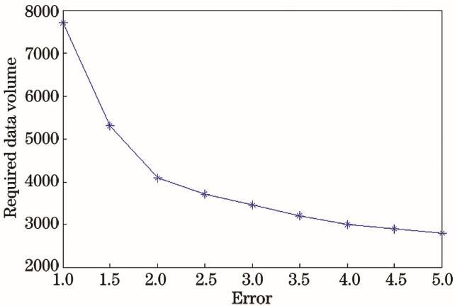
Fig. 1. Relationship between data volume and error
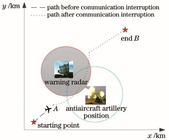
Fig. 2. Battlefield scenario of UAV threat assessment
Fig. 3. UAV threat assessment framework diagram
Fig. 4. BN structure matrix expression
Fig. 5. Construction flow chart of the constraint matrix
Fig. 6. Flow chart of BN structure learning algorithm based on matrix constraints
Fig. 7. Flow chart of parameter learning algorithm based on prior constraints
Fig. 8. Total BIC score of the algorithm proposed in this paper and the K2 algorithm
Fig. 9. Average BIC score of the algorithm proposed in this paper and K2 algorithm
Fig. 10. Total Hamming distance between the algorithm in this paper and the K2 algorithm
Fig. 11. Average Hamming distance between the algorithm in this paper and the K2 algorithm
Fig. 12. Threat assessment network based on 20 sets of data by our algorithm
Fig. 13. Threat assessment network based on 30 sets of data by our algorithm
Fig. 14. Threat assessment network based on 40 sets of data by our algorithm
Fig. 15. Threat assessment network based on 50 sets of data by our algorithm
Fig. 16. UAV threat assessment network model structure
Fig. 17. Threat assessment network derived from 40 sets of data by K2 algorithm
Fig. 18. Threat assessment network derived from 50 sets of data by K2 algorithm
Fig. 19. Threat assessment network derived from 60 sets of data by K2 algorithm
Fig. 20. Threat assessment network derived from 70 sets of data by K2 algorithm
Fig. 21. Relationship between data volume and threat probability
|
Table 1. Discretization of target node information
| |||||||||||||||
Table 2. Interval constraints corresponding to parameters
| |||||||||||||||
Table 3. Initial parameters of threat assessment model
| |||||||||||||||
Table 4. 40 sets of data model parameters obtained by our algorithm
| |||||||||||||||
Table 5. 50 sets of data model parameters obtained from our algorithm
| |||||||||||||||
Table 6. 60 sets of data model parameters obtained by our algorithm
| |||||||||||||||
Table 7. Model parameters obtained from 60 sets of data by MLE algorithm
| |||||||||||||||
Table 8. Model parameters obtained from 70 sets of data by MLE algorithm
| |||||||||||||||
Table 9. Model parameters obtained from 80 sets of data by MLE algorithm
|
Table 10. KL-divergence results of this algorithm
|
Table 11. KL-divergence results of MLE algorithm

Set citation alerts for the article
Please enter your email address
© Copyright 2018-2021 | Chinese Laser Press. All Rights Reserved 沪ICP备15018463号-20