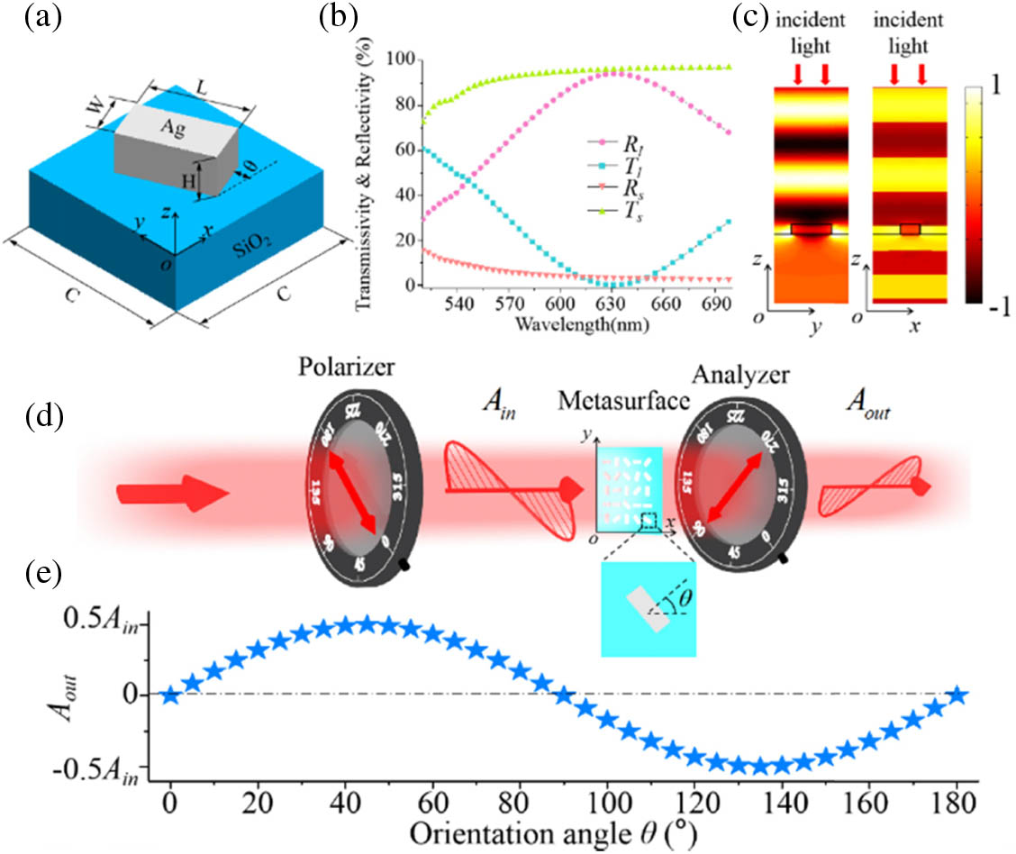
Fig. 1. Illustration of both positive and negative amplitude modulation of the nanobrick-based metasurface. (a) Schematic of a nanobrick unit cell. The nanobrick can be rotated in the xoy plane with an orientation angle θ. (b) Transmissivity and reflectivity versus wavelength (520–700 nm), where s and l denote the polarization directions of the normally incident light along the short and long axes of the nanobrick, respectively. (c) Electric field distribution in the nanostructure with incident light polarized along the long or short axis, respectively. The orientation angle θ in (b) and (c) is 0°. (d) Illustration of the optical setup for continuous amplitude modulation. (e) Output light amplitudes versus orientation angles.

Fig. 2. Comparison of a conventional digital hologram with a zero-order-free meta-hologram. (a) A conventional digital hologram with amplitude distribution in an interval of [0,1]. (b) An enlarged view of the partial amplitude distribution. (c) The 3D intensity distribution of the reconstructed image containing strong zero-order light. (d) A zero-order-free meta-hologram with amplitude distribution in an interval of [−0.5, 0.5]. (e) An enlarged view of the partial amplitude distribution. (f) The 3D intensity distribution of the holographic image without the zero-order light.

Fig. 3. Schematic of experimental setup, simulated amplitude distribution, and experimental results for the zero-order-free meta-hologram. (a) Schematic diagram of decoding the meta-hologram in the far field. (b) Simulated amplitude distribution with 2×2 periods. (c) Enlarged amplitude distribution (100×100 pixels) of the white dashed box shown in (b). (d) Partial SEM image of the fabricated sample (top view). (e) Intensity distribution (one period of the meta-hologram) at the surface of the sample captured by an optical microscope with a magnification of 50. (f) Experimentally obtained holographic image under the illumination of a normally incident laser source (632.8 nm). Solid and dashed lines at the top right represent the transmission axes of the polarizer and analyzer, respectively. (g) Partial zoom-in view of (f).

Fig. 4. Holographic images generated by illuminating the zero-order-free meta-hologram with a supercontinuum laser source ranging from 520 to 660 nm in steps of 20 nm. The solid and dashed lines at the top right of the image represent the transmission axes of the polarizer and analyzer, respectively.