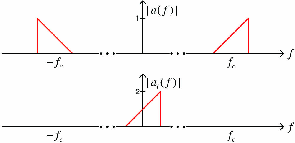
Fig. 1. Spectrum of the modulated optical signal (top) and its baseband equivalent signal (bottom).

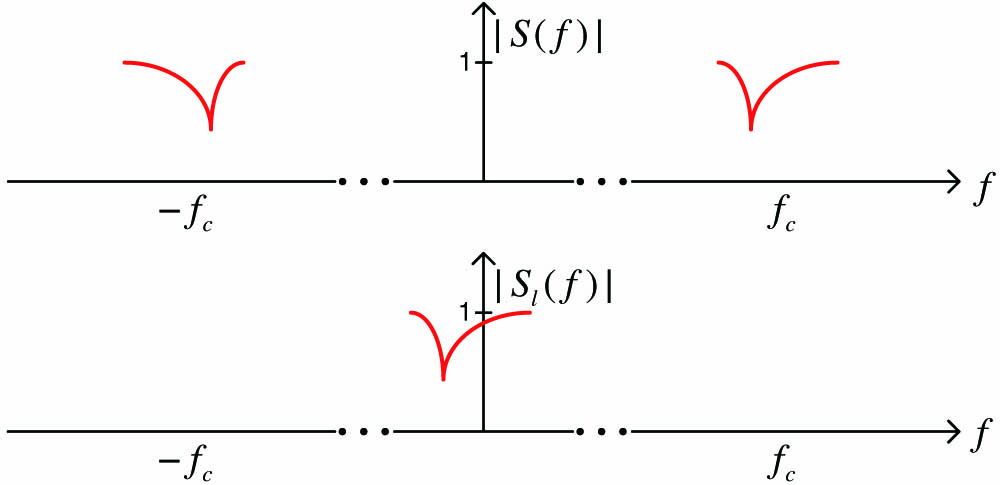
Fig. 2. Spectrum of bandpass systems (top) and the corresponding baseband equivalent systems (bottom).

Fig. 3. The simulated or measured scattering parameters at a set of discrete frequency samples (top) and the corresponding baseband scattering parameters (bottom).

Fig. 4. Flow chart of the CVF modeling approach (left branch) and the one presented in Ref. [12] (right branch).

Fig. 5. Spectrum of the model SVF(f) (top) and the model SlVF(f) represented by Model (9) (bottom).

Fig. 6. Poles of the model SVF(f) (left) and the model SlVF(f) represented by Model (9) (right).

Fig. 7. Example 7.A. The structure of the five-ring resonator filter.

Fig. 8. Example 7.A. The accuracy of the VF-based Model (9) (top) built via the technique in Ref. [12] with 108 poles and the CVF Model (6) (bottom) built via the newly proposed technique with 54 poles; the red solid lines represent the simulated scattering parameters, the blue dashed lines represent the models, while the green lines are the magnitude of the error between the two.

Fig. 9. Example 7.A. The poles of the CVF Model (6) from the proposed technique (represented by circles) and the VF-based Model (9) from the technique in Ref. [12] (represented by crosses).

Fig. 10. Example 7.A. The in-phase part I(t) and quadrature part Q(t) of the 16 QAM input signal.

Fig. 11. Example 7.A. The output signals at P1, P2, P3, and P4 obtained from baseband time-domain simulations of Models (6), (9), and (14).

Fig. 12. Example 7.A. Constellation diagrams of the transmission signal at P3 calculated from different models.

Fig. 13. Example 7.B. The schematic circuit of the ring-loaded MZI filter.

Fig. 14. Example 7.B. The accuracy of the VF-based Model (9) (top) built via the technique in Ref. [12] with 42 poles and the CVF Model (6) (bottom) built via the newly proposed technique with 21 poles; the red solid lines represent the simulated scattering parameters, and the blue dashed lines represent the models, while the green lines are the magnitude of the error between the two.

Fig. 15. Example 7.B. The poles of the CVF Model (6) (represented by circles) and the Model (9) from the VF-based technique in Ref. [12] (represented by crosses).

Fig. 16. Example 7.B. The output signals at P3 and P4 obtained from baseband time-domain simulation of Models (6), (9), and (14).

Fig. 17. Example 7.B. Constellation diagram of the transmission signal at P3 calculated from different models.

Fig. 18. Example 7.B. Constellation diagram of the transmission signal at P3 calculated from the rebuilt CVF Model (6) and the shifted Model (21), when the passband of the filter redshifts and blueshifts by 0.3 nm.

Fig. 19. Example 7.C. The structure of the Mach–Zehnder interferometer lattice filter.

Fig. 20. Example 7.C. The singular values of the scattering matrices calculated from Model (6) before and after passivity enforcement.

Fig. 21. Example 7.C. The accuracy of the VF-based Model (9) (top) built via the technique in Ref. [12] with 68 poles and the new CVF Model (6) with 34 poles (bottom); the red solid lines represent the simulated scattering parameters, and the blue dash lines represent the models, while the green lines show the error between them.