Time-domain compact macromodeling of linear photonic circuits via complex vector fitting

Yinghao Ye; Domenico Spina; Dirk Deschrijver; Wim Bogaerts; Tom Dhaene

doi:10.1364/PRJ.7.000771

Abstract

In this paper, a novel baseband macromodeling framework for linear passive photonic circuits is proposed, which is able to build accurate and compact models while taking into account the nonidealities, such as higher order dispersion and wavelength-dependent losses of the circuits. Compared to a previous modeling method based on the vector fitting algorithm, the proposed modeling approach introduces a novel complex vector fitting technique. It can generate a half-size state-space model for the same applications, thereby achieving a major improvement in efficiency of the time-domain simulations. The proposed modeling framework requires only measured or simulated scattering parameters as input, which are widely used to represent linear and passive systems. Three photonic circuits are studied to demonstrate the accuracy and efficiency of the proposed technique.

1. INTRODUCTION

Time-domain characterizations of photonic integrated circuits (PICs), such as transient response, bit error rate, and eye diagram, are direct performance metrics of PICs and a basic step for circuit synthesis and signal integrity analysis. With years of improvement of photonic simulation software tools, nowadays such time-domain characterizations mainly depend on the accuracy and efficiency of the circuit models of the PIC components ^[1].

A range of models for active photonic components has been presented in the literature (e.g., lasers ^[2–4], modulators ^[5–7], photodetectors ^[8–10]). However, for passive components [e.g., directional couplers (DCs), wavelength filters], which are usually described in the frequency domain, few publications discuss how to build accurate and efficient time-domain models for circuit simulations ^[11–13]. Actually, if imperfections such as higher order dispersion, wavelength-dependent losses, and imperfections in coupling coefficients are ignored during the modeling phase, it is not difficult to derive time-domain models of passive components, as demonstrated in Refs. ^[14,15]. Nevertheless, these imperfections may considerably affect the behaviors of PICs and can often not be overlooked, especially for complex devices such as wavelength filters.

The passive components in PICs share a common feature: their behavior can be fully represented in the frequency domain by scattering parameters that are able to capture the aforementioned nonidealities. Therefore, it is convenient and accurate to conduct time-domain simulations starting from these scattering parameters. It is intuitive to directly apply inverse fast Fourier transform to scattering parameters to obtain the corresponding impulse response, and then time-domain simulations can be performed by a convolution with inputs. But in practice, the scattering parameters are band-limited or truncated, and this method often leads to violations of physical properties ^[16], such as causality and passivity. In Ref. ^[11], the finite impulse response (FIR) modeling technique for time-domain simulation takes advantage of scattering parameters and is adopted in the photonic simulator Lumerical INTERCONNECT ^[17]. However, the accuracy provided by FIR filters substantially depends on the design methodology employed, and it inherently degrades near the edges of the simulated signal bands ^[11]. Another approach is to build a baseband state-space model ^[12,13] from the scattering parameters via the robust vector fitting (VF) technique ^[18–20], which is extensively used in the electronic domain to model distributed microwave devices. Such a model is inherently a system of first-order ordinary differential equations (ODEs) and can be efficiently simulated in ODE solvers ^[12,13].

Sign up for Photonics Research TOC. Get the latest issue of Photonics Research delivered right to you！Sign up now

In this work, a novel alternative approach is presented, called complex vector fitting (CVF), which preserves all the advantages of the previous methods in Refs. ^[12,13], but generates more compact baseband state-space models that are only half the size of the corresponding models obtained via Refs. ^[12,13]. Note that this reduces the simulation time by, at least, a factor of 2 ^[21]. This is a significant advantage when considering complex systems with a large number of passive components. However, the proposed models are complex-valued state-space systems and can only be adopted in simulators supporting complex-valued signals and matrices. Since many solver techniques are developed and optimized for real-valued systems, such as SPICE and Verilog-A, it is demonstrated that such a stable and passive complex-valued baseband model can be directly converted into a corresponding real-valued state-space representation, whose stability and passivity are preserved by construction. It is important to note that the proposed CVF-based modeling technique is significantly different from the previous works ^[12,13] that are based on the VF technique. The differences are deeply discussed in the paper, and their impact on simulation time is also demonstrated.

The paper is organized as follows. Section 2 presents an overview on baseband signals and systems. The novel compact baseband modeling approach is presented in Section 3, while its passivity assessment and enforcement are studied in Section 4. Section 5 compares the proposed technique with the previous ones in Refs. ^[12,13]. The real-valued baseband model is derived in Section 6, and its properties are rigorously discussed. Finally, Section 7 presents three photonic circuits examples, and conclusions are drawn in Section 8.

2. PROBLEM STATEMENT

Photonic circuits are characterized in the optical frequency range: for telecommunication applications, this is typically defined as [187;200] THz, which corresponds to wavelengths in the range of [1.5;1.6] μm. A direct time-domain simulation in this overwhelmingly high frequency range is impractical in terms of computational time and memory requirements ^[12,15], especially for large and complex PICs. In particular, the transmitted signals in photonic systems are usually defined as amplitude and/or phase-modulated optical signals in the form where $f_{c}$ is the optical carrier frequency, while $A (t)$ and $ϕ (t)$ are the time-varying amplitude and phase, respectively, which are radio frequency (RF) modulating signals. Hence, the spectrum of $a (t)$ is centered around the optical carrier frequency, and its bandwidth is relatively small compared to $f_{c}$ . The signals in form (1) are called bandpass signals ^[22]. Analogously, general linear and passive photonic circuits that deal with signals in form (1) can be considered as bandpass systems.

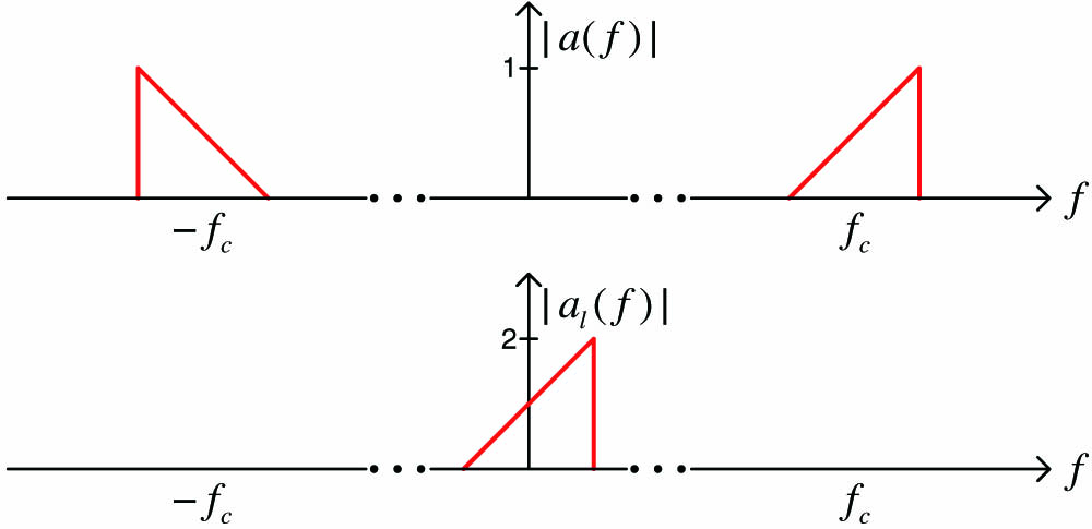
In this scenario, time-domain simulations of bandpass photonic circuits have to be carried out with very small time steps due to the large carrier frequency, whereas the baseband modeling and simulation approach can adopt relatively large time steps to significantly increase the efficiency without losing accuracy ^[12,22]. The main idea is to “remove” the optical carrier frequency from the bandpass signal $a (t)$ by deriving a corresponding baseband equivalent signal $a_{l} (t)$ as ^[22] which represents the complex envelope of the signal $a (t)$ . The relation between $a (t)$ and $a_{l} (t)$ in the frequency domain is more intuitive and is illustrated in Fig. 1. The baseband equivalents for bandpass systems can be defined in a similar way, shown in Fig. 2, where $S (f)$ is the frequency response of the bandpass system, while $S_{l} (f)$ is its baseband equivalent. If $a (t)$ is the port signal of the bandpass system $S (f)$ , $a_{l} (t)$ can be considered as the port signal of the baseband equivalent system $S_{l} (f)$ . Interested readers are referred to Ref. ^[22] for more details about the definition and derivation of baseband equivalent signals and systems. One important property of the baseband modeling and simulation approach is that the port signals [in the form (1)] of the bandpass photonic circuits can be analytically recovered from their baseband equivalents [in the form (2)] ^[12,22].

Spectrum of the modulated optical signal (top) and its baseband equivalent signal (bottom).

Figure 1.Spectrum of the modulated optical signal (top) and its baseband equivalent signal (bottom).

Figure 2.Spectrum of bandpass systems (top) and the corresponding baseband equivalent systems (bottom).

It is easy to observe that $S_{l} (f)$ is simply equal to $S (f)$ at the positive frequencies shifted by $- f_{c}$ . As shown in Fig. 2, $S_{l} (f)$ is a mathematical representation of a physical system that has an asymmetric frequency response with regard to the positive and negative frequencies. Therefore, it also has a complex-valued impulse response in the time domain. Directly computing a model of $S_{l} (f)$ that can be used for time-domain simulation is a challenging problem. In the next two sections, a novel methodology to compute stable and passive baseband models of $S_{l} (f)$ in state-space form is proposed.

3. POLE-RESIDUE MODELING VIA COMPLEX VECTOR FITTING

As described in Section 1, the modeling process starts from the scattering parameters in order to take into account nonideal behaviors such as higher order dispersion and wavelength-dependent losses. Hence, let us assume that the scattering parameters of the photonic circuit under study have been obtained (via simulations or measurements) for a discrete set of frequency values in the bandwidth of interest for the application considered: $S (f_{r})$ for $r = 1, \dots, R$ .

Next, shifting $S (f_{r})$ towards 0 Hz by the carrier frequency $f_{c}$ leads to the baseband scattering parameters $S_{l} (f_{i})$ , as shown in Fig. 3, where $f_{i} = f_{r} - f_{c}$ . Then, the CVF algorithm is developed to calculate a pole-residue model of $S_{l} (f_{i})$ as where $s = j 2 π f$ is the Laplace variable, $p_{k}$ are the (common) poles, which can be either real or complex, and $R_{k}$ are the corresponding residues, while $D$ is a real matrix. This form is very similar to pole-residue models that can be computed by the well-known VF algorithm ^[18,19], which was proposed two decades ago and is widely used in the electronic field to build pole-residue models for linear passive-distributed devices and systems represented by scattering parameters. There are several versions of the VF algorithm that adopt different modeling strategies ^[18,23,24] and passivity enforcement methods ^[20,25–28]. In this work, the CVF is a variant of the VF algorithm available in Ref. ^[29], which implements the techniques in Refs. ^[18–20,30]. Since VF has been extensively studied in the past two decades, and the proposed CVF shares several similarities with it, only the differences between them that are relevant for our application will be discussed. Interested readers are referred to Refs. ^[18–20,30] for a thorough understanding of the VF modeling approach.

Figure 3.The simulated or measured scattering parameters at a set of discrete frequency samples (top) and the corresponding baseband scattering parameters (bottom).

In particular, both CVF and VF adopt pole-residue models formed by real and complex poles having a negative real part, in order to guarantee the stability of the model ^[31]. However, the complex poles and the corresponding residues computed via VF must always occur in complex conjugate pairs, for example, where $k$ is the pole and residue index in Model (3), $α$ is a real positive scalar forcing all the poles in left-hand side of the complex plane (for stability), and $β$ is a (positive or negative) real scalar, while $η$ and $γ$ are real matrices.

The frequency response of physical linear systems is always symmetric about zero (even amplitude and odd phase). The complex conjugate constraint on poles (and residues) implemented in VF allows to preserve this property, such that the corresponding impulse response in the time domain is guaranteed to be real-valued. However, baseband systems are nonphysical and have an asymmetric frequency response with respect to 0 Hz by construction. Therefore, VF cannot be applied to modeling such a system directly ^[12,13], as described in Section 5.

In order to overcome this problem, the complex conjugacy constraint on poles (and residues) is removed in the CVF algorithm. Besides this difference, the methodology employed to compute a pole-residue model is the same: the pole flipping scheme ^[18], relaxed formulation ^[30], and fast implementation based on QR decomposition ^[19] used in VF can be directly adopted for CVF.

The idea of removing the complex conjugacy constraint in the VF algorithm was first proposed in Refs. ^[32,33] in order to design complex infinite impulse response (IIR) filters having asymmetric frequency response. There are two important differences with regard to this work. (1) The $D$ matrix in Ref. ^[32] is assumed to be a complex matrix, whereas it must be real in this work. This physics-based restriction is relevant for our applications, as discussed in Section 6.B. (2) The models built in Ref. ^[32] are not used for time-domain simulations: the passivity definition, assessment, and enforcement of the complex-valued models are not investigated in Ref. ^[32], while here they are rigorously studied in Section 4.

Once a Model (3) has been obtained via the CVF algorithm, it can be easily converted into a corresponding state-space form ^[34] as where $a_{l} (t) \in C^{n \times 1}$ and $b_{l} (t) \in C^{n \times 1}$ are the input and output signals of the $n$ -port baseband system, respectively, which are the baseband equivalents of the modulated port signals of the original photonic circuit, while $x_{l} (t) \in C^{m \times 1}$ with $m = n K$ collects the state variables. The matrices $A$ , $B$ , $C$ , $D$ can be analytically derived from Model (3): $A \in C^{m \times m}$ is a diagonal matrix with all the poles $p_{k}$ as diagonal entries, $B \in R^{m \times n}$ is a matrix containing only ones and zeros, $C \in C^{n \times m}$ contains all the residues $R_{k}$ , and $D \in R^{n \times n}$ is the same as in Model (3) ^[34]. Model (6) offers two main advantages: •

fundamental properties for time-domain simulations, such as causality, stability, and passivity, are well defined for state-space models;

•

state-space models are systems of first-order ODEs: time-domain simulations can be performed by solving the state-space models in a variety of robust ODE solvers with great accuracy and efficiency, for example, the MATLAB linear state-space system solver lsim.

It is important to remark that the computational time for building a CVF model with $K$ poles is comparable to the time needed to build a VF model with $2 K$ poles. The number of unknowns is the same in both algorithms, considering that the poles and residues in VF are complex conjugated ^[18].

4. PASSIVITY ASSESSMENT AND ENFORCEMENT OF CVF MODELS

Since the baseband Model (6) will be used for simulations in the time domain, the model passivity must be checked and, eventually, enforced ^[31]. In Ref. ^[12], the passivity definition and conditions for complex-valued linear baseband systems are presented. In particular, there are two passivity constraints that the baseband scattering parameters $S_{l} (s)$ must satisfy: 1.

$S_{l} (s)$ is analytic in $R (s) > 0$ ;

$I_{n} - S_{l}^{H} (s) S_{l} (s)$ is a nonnegative-definite matrix for all $s$ such that $R (s) > 0$ ,

where

R (s)

represents the real part of the Laplace variable, while

I_{n}

is the identity matrix of size

n \times n

. Note that such conditions are the same as for physical systems, with the exception that the conjugacy relation

S^{*} (s) = S (s^{*})

no longer needs to hold for complex-valued systems.

Now, the above passivity conditions require that the maximum singular value of $S_{l} (s)$ is bounded by unity at all frequencies. In this framework, it has been proven that the Hamiltonian matrix $M$ can be used to assess the model passivity with accuracy and efficiency ^[12], which is defined as where Note that $M_{11}$ , $M_{21}$ , $M_{22}$ are complex matrices, while $M_{12}$ is real, since $A$ and $C$ are complex, while $B$ and $D$ are real. The Hamiltonian matrix for complex-valued systems is very similar to the corresponding one defined for real-valued ones, except that the former employs the conjugate transpose operator $H$ ^[12], whereas the latter one can use the transpose operator $T$ ^[34], as shown in Section 6.B.

In particular, a (complex- or real-valued) stable state-space model is passive if its Hamiltonian matrix has no purely imaginary eigenvalues: any such eigenvalue indicates a crossover frequency where a singular value of the scattering matrix changes from being smaller to larger than unity, or vice versa ^[12,34]. Once the crossover frequency points are identified by checking the eigenvalues of the Hamiltonian matrix (7), the local maxima of violating singular values of the scattering matrix can be found ^[20]. Passivity can be enforced by perturbing the residues such that the violating singular values become smaller than unity ^[20].

From an algorithmic point of view, the CVF technique offers a robust model building tool and can leverage on powerful passivity assessment and enforcement techniques developed for the VF algorithm, with one exception. Indeed, the half-size passivity test matrix that is proposed in Ref. ^[34] for an efficient passivity assessment of real-valued reciprocal systems is no longer applicable to the complex-valued systems studied in this paper, due to the presence of the conjugate transpose operator $H$ in the Hamiltonian matrix (7). Interested readers are referred to Ref. ^[34] for details.

5. COMPARISON WITH PREVIOUS WORK

Recently, a baseband macromodeling strategy based on pole-residue models has been presented in Refs. ^[12,13]. The main differences with respect to the proposed modeling framework are outlined in Fig. 4. In particular, the approach in Ref. ^[12] is based on the VF algorithm: first a state-space model $S^{VF} (f)$ of $S (f_{r})$ is computed via VF. Then, since $S^{VF} (f)$ operates in the optical frequency range, it is converted into a baseband model $S_{l}^{VF} (f)$ , whose time-domain state-space representation is in the form where $A_{VF}, B_{VF}, C_{VF}, D_{VF}$ are the state-space matrices of $S^{VF} (f)$ computed via VF, starting from the bandpass scattering parameters $S (f_{r})$ . In particular, $A_{VF}$ is a diagonal matrix containing the real or complex conjugate poles identified by VF, $C_{VF}$ is a matrix that contains residues, $B_{VF}$ is a matrix containing only ones and zeros, and $D_{VF}$ is a real-valued matrix. Whereas the CVF Model (6) and VF-based Model (9) are somewhat similar, the different modeling strategies result in a major difference: the novel proposed approach allows one to build a model that can have half the size of the Model (9) in terms of number of poles and state variables, thereby significantly decreasing the simulation time. The reason is clearly identified by considering the frequency-domain response $S_{l}^{VF} (f)$ of Model (9).

Figure 4.Flow chart of the CVF modeling approach (left branch) and the one presented in Ref. [12] (right branch).

Indeed, the frequency response $S_{l}^{VF} (f)$ has also components around $- 2 f_{c}$ , since it is computed by shifting the VF model $S^{VF} (f)$ defined at bandpass frequency, as indicated in Fig. 5. In particular, by looking at Model (9), the poles of the VF model $S^{VF} (f)$ collected in the matrix $A_{VF}$ are shifted by the quantity $- j 2 π f_{c}$ , as shown in the complex plane in Fig. 6. Clearly, the poles around $- j 4 π f_{c}$ do not contribute to the results of time-domain simulations performed with baseband signals $a_{l} (t)$ defined around 0 Hz (see Fig. 1). Intuitively, the frequency response around $- 2 f_{c}$ can be removed by simply discarding the corresponding poles and residues from Model (9), thereby achieving a half-size compact model. However, this brute-force operation can cause two problems: 1) slightly decreasing the accuracy of the desired frequency response around 0 Hz and 2) accidentally turning Model (9) from passive to nonpassive. So, calculation of the half-size Model (6) using the CVF technique is advised.

Figure 5.Spectrum of the model $S^{VF} (f)$ (top) and the model $S_{l}^{VF} (f)$ represented by Model (9) (bottom).

Figure 6.Poles of the model $S^{VF} (f)$ (left) and the model $S_{l}^{VF} (f)$ represented by Model (9) (right).

For time-domain simulations, solving the half-size Model (6) requires less than half of the computational complexity with respect to Model (9). For example, the two main steps in the MATLAB routine lsim to solve a linear system of ODEs have a computational complexity of $O (m^{3})$ and $O (m^{2} N_{t})$ ^[21], respectively, where $m = n K$ is the size of $A$ and $N_{t}$ is the total number of time samples. Hence, the proposed technique offers a significant computational advantage, especially when the model size is large.

6. REAL-VALUED BASEBAND STATE-SPACE MODELS

Both the baseband CVF Model (6) and the VF-based Model (9) are complex-valued systems and can be simulated only in solvers that support complex-valued signals and matrices. However, in Ref. ^[13], the VF-based Model (9) is analytically converted to a real-valued model that can be adopted in a wider range of simulators, such as SPICE and Verilog-A. In this section, we will demonstrate that a real-valued baseband state-space model can also be derived, starting from the CVF modeling framework described in Section 3. Additionally, its stability and passivity properties are investigated.

A. Model Derivation

Complex signals can be represented as a sum of their real and imaginary parts, such as for $a_{l} (t)$ , $a_{l} (t) = a_{l R} (t) + j a_{l I} (t) .$ (10)Note that for a quadrature amplitude modulation (QAM) signal, $a_{l R} (t)$ and $a_{l I} (t)$ can be considered as in-phase and quadrature parts, respectively ^[12,13]. Expressing all the complex signals and matrices in Model (6), namely $a_{l} (t)$ , $b_{l} (t)$ , $x_{l} (t)$ , $A$ , and $C$ , in the form (10) and solving separately with respect to the real and the imaginary parts leads to ${\begin{matrix} \frac{d x_{l R} (t)}{d t} = A_{R} x_{l R} (t) - A_{I} x_{l I} (t) + {Ba}_{l R} (t), \\ \frac{d x_{l I} (t)}{d t} = A_{R} x_{l I} (t) + A_{I} x_{l R} (t) + {Ba}_{l I} (t), \\ b_{l R} (t) = C_{R} x_{l R} (t) - C_{I} x_{l I} (t) + {Da}_{l R} (t), \\ b_{l I} (t) = C_{R} x_{l I} (t) + C_{I} x_{l R} (t) + {Da}_{l I} (t), \end{matrix}$ (11)where the indexes $R$ and $I$ indicate the real and imaginary parts, respectively. Then, by defining $\hat{a} (t) = [\begin{matrix} a_{l R} (t) \\ a_{l I} (t) \end{matrix}], \hat{b} (t) = [\begin{matrix} b_{l R} (t) \\ b_{l I} (t) \end{matrix}], \hat{x} (t) = [\begin{matrix} x_{l R} (t) \\ x_{l I} (t) \end{matrix}],$ (12)and $\begin{matrix} \hat{A} = [\begin{matrix} A_{R} & - A_{I} \\ A_{I} & A_{R} \end{matrix}], & \hat{B} = [\begin{matrix} B & 0 \\ 0 & B \end{matrix}], \\ \hat{C} = [\begin{matrix} C_{R} & - C_{I} \\ C_{I} & C_{R} \end{matrix}], & \hat{D} = [\begin{matrix} D & 0 \\ 0 & D \end{matrix}], \end{matrix}$ (13)where 0 represents the null matrix, Eq. (11) can be written as ${\begin{matrix} \frac{d \hat{x} (t)}{d t} = \hat{A} \hat{x} (t) + \hat{B} \hat{a} (t) \\ \hat{b} (t) = \hat{C} \hat{x} (t) + \hat{D} \hat{a} (t), \end{matrix}$ (14)which is defined as real-valued baseband state-space model.

It is important to remark the main difference of the real-valued representation [Model (14)] with respect to the complex-valued one [Model (6)]. Model (6) is a purely mathematical representation of the system under study, as described in Section 2. The novel Model (14) has a symmetrical frequency response with respect to the positive and negative frequencies, and its impulse response and input and output signals are real. Hence, it represents a physical linear system, while it can still be simulated at baseband. Furthermore, the novel Model (14) is also a system of first-order real-valued ODEs. Hence, it can be solved in a wider range of simulators than the complex-valued Model (6).

B. Stability and Passivity Analysis

Since Model (14) can be considered as a physical, linear, and time-invariant system, the stability and passivity conditions defined for physical linear systems ^[31] still hold for the new Model (14).

The stability of a state-space model can be assessed from the eigenvalue of the matrix $\hat{A}$ : the model is stable if the real part of all the eigenvalues is negative ^[31].

First, a similarity transformation is applied to $\hat{A}$ , $\tilde{A} = T^{- 1} \hat{A} T = [\begin{matrix} A_{R} - j A_{I} & 0 \\ 0 & A_{R} + j A_{I} \end{matrix}] = [\begin{matrix} A^{*} & 0 \\ 0 & A \end{matrix}],$ (15)where $T = [I_{m}, I_{m}; j I_{m}, - j I_{m}]$ . If all the eigenvalues of $A$ are in the vector $λ$ , then Eq. (15) indicates that the eigenvalues of $\tilde{A}$ are $λ$ and $λ^{*}$ combined. Since similarity transformations do not change the eigenvalues, $\tilde{A}$ and $\hat{A}$ share the same set of eigenvalues. Therefore, when the CVF Model (6) is stable (all the elements in $λ$ have negative real parts), the real-valued Model (14) is stable as well (all the eigenvalues of $\hat{A}$ have negative real parts).

Then, as indicated in Section 4, the passivity of Model (14) can be verified by means of the Hamiltonian matrix for real-valued models ^[34], $\hat{M} = [\begin{matrix} {\hat{M}}_{11} & {\hat{M}}_{12} \\ {\hat{M}}_{21} & {\hat{M}}_{22} \end{matrix}],$ (16)where ${\hat{M}}_{11} = \hat{A} - \hat{B} {\hat{L}}^{- 1} {\hat{D}}^{T} \hat{C}, {\hat{M}}_{12} = - \hat{B} {\hat{L}}^{- 1} {\hat{B}}^{T}, {\hat{M}}_{21} = {\hat{C}}^{T} {\hat{Q}}^{- 1} \hat{C}, {\hat{M}}_{22} = - {\hat{A}}^{T} + {\hat{C}}^{T} \hat{D} {\hat{L}}^{- 1} {\hat{B}}^{T}, \hat{L} = {\hat{D}}^{T} \hat{D} - I_{2 n}, \hat{Q} = \hat{D} {\hat{D}}^{T} - I_{2 n} .$ (17)Starting from Eqs. (13), (8), and (17), after some block matrix calculations described in Appendix A, the following relations can be derived: $\begin{matrix} {\hat{M}}_{11} = [\begin{matrix} M_{11}^{R} & - M_{11}^{I} \\ M_{11}^{I} & M_{11}^{R} \end{matrix}], \end{matrix} \begin{matrix} {\hat{M}}_{12} = [\begin{matrix} M_{12} & 0 \\ 0 & M_{12} \end{matrix}], \end{matrix} \begin{matrix} {\hat{M}}_{21} = [\begin{matrix} M_{21}^{R} & - M_{21}^{I} \\ M_{21}^{I} & M_{21}^{R} \end{matrix}], \end{matrix} \begin{matrix} {\hat{M}}_{22} = [\begin{matrix} M_{22}^{R} & - M_{22}^{I} \\ M_{22}^{I} & M_{22}^{R} \end{matrix}], \end{matrix}$ (18)where $M_{11}^{R}$ and $M_{11}^{I}$ are the real and imaginary parts of $M_{11}$ , respectively, and the same notation is also adopted for $M_{12}$ , $M_{21}$ , $M_{22}$ . It is important to remark that Eq. (18) can only be derived thanks to the restriction of computing $D$ in Model (3) as the real matrix, as indicated in Section 3.

By performing a similarity transformation on $\hat{M}$ , a new matrix $\bar{M}$ can be obtained, $\bar{M} = P^{- 1} \hat{M} P = [\begin{matrix} M^{*} & 0 \\ 0 & M \end{matrix}],$ (19)where $P = [\begin{matrix} I_{m} & 0 & I_{m} & 0 \\ j I_{m} & 0 & - j I_{m} & 0 \\ 0 & I_{m} & 0 & I_{m} \\ 0 & j I_{m} & 0 & - j I_{m} \end{matrix}],$ (20)and $M$ is the Hamiltonian matrix of the CVF Model (6), described in Eq. (7). Note that the similarity transformation [Eq. (19)] can be derived by simple algebraic manipulations. Since similarity transformations do not change the eigenvalues, the eigenvalues of $\hat{M}$ are the union set of the eigenvalues of $M$ and their complex conjugate according to Eq. (19). This proves that, if the stable Model (6) is passive ( $M$ does not have any purely imaginary eigenvalue), then the real-valued Model (14) is passive by construction ( $\hat{M}$ has no purely imaginary eigenvalue either).

7. EXAMPLES ON PHOTONIC CIRCUITS

This section presents three application examples of the proposed modeling and simulation techniques. The scattering parameters of the photonic circuits under study are evaluated via the Caphe circuit simulator (Luceda Photonics) and electromagnetic simulations in FDTD Solutions (Lumerical), while the time-domain simulations are carried out in MATLAB on a personal computer with Intel Core i3 processor and 8 GB RAM.

A. Five-Ring Resonator Filter

A five-ring resonator filter based on Ref. ^[35] is studied in this section. The filter comprises four DCs and two multimode interferometers (MMIs), as shown in Fig. 7. The geometric parameters of the filter can be found in Ref. ^[35] and will not be repeated here.

Figure 7.Example 7.A. The structure of the five-ring resonator filter.

A direct finite-difference time-domain (FDTD) simulation of the entire five-ring filter is very time consuming, as the structure is very large, and because of the resonances, a very long simulation time is needed to reach the termination condition where the residual fields have died out. Therefore, we only simulate the coupling structures, i.e., the MMI and two DCs (indicated in Fig. 7) given that the filter is symmetric, and evaluate the scattering parameters in the modeling frequency range [187.37;199.86] THz (corresponding to a wavelength range of [1.5;1.6] μm) while considering a carrier frequency $f_{c} = 193.46 THz$ . In this example, 500 frequency samples are used, and they are uniformly distributed over the frequency range of interest. Adaptive sampling strategies can also be adopted to choose the frequency samples efficiently: more samples are chosen where the frequency response is dynamic, such as resonances, and less are chosen in smooth areas ^[31]. Then, the scattering parameters of the whole filter are calculated in the circuit simulator Caphe by connecting the MMI and DCs.

Following the CVF modeling procedure, the evaluated scattering parameters over optical frequency range are first shifted to the baseband $[- 6.09; 6.40] THz$ by $f_{c} = 193.46 THz$ . Next, a stable and passive baseband Model (6) is built with 54 poles. A standard bottom-up approach is used to select the required number of poles ^[31,36]: the initial number of poles is iteratively increased until the desired accuracy is reached. Then, a real-valued state-space Model (14) for the filter is directly derived from Model (6) according to Eq. (13). Note that we deliberately considered a wide-modeling frequency range in order to make the modeling process more challenging, even though RF signals with such large spectrum are rarely used. As a comparison, Model (9) is also built via the VF algorithm with 108 poles. The magnitude of the maximum absolute error for both models is less than $- 52 dB$ , as shown in Fig. 8. Note that the calculated models are already passive, so no passivity enforcement is required in this example. The scattering parameters of the filter are full matrices, since reflections are captured by the FDTD simulator. Hence, even though only $S_{11}$ and $S_{13}$ are shown in Fig. 8 for readability, the model is bidirectional, includes reflections, and can be excited from any of the ports. The poles of Models (6) and (9) are illustrated in Fig. 9. It is clear that half of the poles of Model (9) are around $- j 4 π f_{c}$ , while the other half cluster around 0 Hz, as explained in Section 5 (see Fig. 6). It is important to remark that the poles of the CVF Model (6) and VF-based Model (9) around 0 Hz are relatively close in the complex plane, but are different: the CVF model is not the same as first computing the VF-based model and then removing the poles around $- j 4 π f_{c}$ .

Figure 8.Example 7.A. The accuracy of the VF-based Model (9) (top) built via the technique in Ref. [12] with 108 poles and the CVF Model (6) (bottom) built via the newly proposed technique with 54 poles; the red solid lines represent the simulated scattering parameters, the blue dashed lines represent the models, while the green lines are the magnitude of the error between the two.

Figure 9.Example 7.A. The poles of the CVF Model (6) from the proposed technique (represented by circles) and the VF-based Model (9) from the technique in Ref. [12] (represented by crosses).

To perform time-domain simulations, we apply a 16 QAM input signal at port P1. The corresponding in-phase $I (t)$ and quadrature component $Q (t)$ are RF bit sequence signals, with bit rate 80 Gbit/s and 1000 bits long. The first 25 bits of $I (t)$ and $Q (t)$ are shown in Fig. 10. Note that $I (t)$ and $Q (t)$ can be considered as the real and imaginary parts of the baseband signals in the form (2), and can be directly adopted for baseband time-domain simulations with Models (6), (9), and (14) ^[12]. Relevant time-domain simulation results obtained by the three models are shown in Fig. 11. Additionally, the transmission signal at P3 (drop port of the filter) is plotted as a constellation diagram to better observe the influence of the filter on the input signal, as shown in Fig. 12. It is demonstrated by Figs. 8, 11, and 12 that the proposed technique is accurate in both frequency and time domains.

Figure 10.Example 7.A. The in-phase part $I (t)$ and quadrature part $Q (t)$ of the 16 QAM input signal.

Figure 11.Example 7.A. The output signals at P1, P2, P3, and P4 obtained from baseband time-domain simulations of Models (6), (9), and (14).

Figure 12.Example 7.A. Constellation diagrams of the transmission signal at P3 calculated from different models.

The model building times of the VF-based Model (9) and the CVF Model (6), are 3.4 s and 3.3 s, respectively. The simulation of the VF-based Model (9), the CVF Model (6), and the real-valued state-space Model (14) requires 132 s, 12 s, and 12 s, respectively: the half-size CVF Model (6) is superior to the full-sized VF-based Model (9) in terms of computational speed, while achieving a comparable accuracy. Note that Models (6) and (14) are mathematically equivalent and can be converted to each other, and they have same number of real-valued unknown variables in the state vector to solve. The computational time for these two models is comparable when the MATLAB routine lsim is employed. However, this is not generally guaranteed for all ODE solvers, which depends on the algorithm implementations in the solver adopted.

B. Ring-Loaded Mach–Zehnder Filter

A ring-loaded Mach–Zehnder interferometer (MZI) filter is designed according to the structure proposed in Ref. ^[37], as shown in Fig. 13. There are six DCs and four ring resonators with a phase shifter (PS) in each ring. The power coupling coefficients and PS parameters are indicated in Fig. 13. Once the PSs are tuned to the desired values, they are kept fixed, and the filter can be considered as a linear time-invariant system. It is important to remark that the filter is designed intentionally to have an asymmetric passband feature, as shown in Fig. 14, which can occur in practice due to the tolerances of the manufacturing process or variations in the tuning of the PSs. In this example, we will demonstrate that the proposed modeling technique is robust with regard to this kind of imperfection as well.

Figure 13.Example 7.B. The schematic circuit of the ring-loaded MZI filter.

Figure 14.Example 7.B. The accuracy of the VF-based Model (9) (top) built via the technique in Ref. [12] with 42 poles and the CVF Model (6) (bottom) built via the newly proposed technique with 21 poles; the red solid lines represent the simulated scattering parameters, and the blue dashed lines represent the models, while the green lines are the magnitude of the error between the two.

The filter is simulated in the Caphe circuit simulator to extract the scattering parameters at 700 equidistantly spread frequency samples within the chosen frequency range [190.34;192.05] THz, which covers a bandwidth of 1710 GHz. The carrier frequency is set at the center of the passband of the filter, $f_{c} = 191.19 THz$ . Note that reflections are not considered in the models of the waveguides and the couplers: the overall circuit has no reflections as well. As a result, the scattering matrices are sparse. The frequency range is chosen to be wide in order to demonstrate the modeling power of the proposed technique. In practice, however, it can be chosen according to the spectrum of the input signals ^[12]. Then, a compact state-space Model (6) is built via the CVF technique with 21 poles over the corresponding baseband frequency range [−850;860] GHz. Finally, the real-valued state-space Model (14) is analytically calculated, as described in Section 6. For comparison, the VF-based Model (9) of the filter is also built via the VF algorithm with 42 poles. The magnitude of the maximum absolute error for both Models (6) and (9) is less than $- 56 dB$ , as shown in Fig. 14. The poles of the CVF Model (6) and the VF-based Model (9) are illustrated in Fig. 15, which again demonstrates the poles from both models around 0 Hz are slightly different. The passivity assessment (see Section 4) reveals that all the models are passive and suitable for time-domain simulations.

Figure 15.Example 7.B. The poles of the CVF Model (6) (represented by circles) and the Model (9) from the VF-based technique in Ref. [12] (represented by crosses).

In particular, the same 16 QAM signal in Fig. 10 is adopted as input for port P1, with one difference: the data rate is decreased from 80 Gbit/s to 20 Gbit/s, since the (single-side) passband of the filter in this example is approximately 50 GHz. Time-domain simulations are conducted with the three models, and the results for the first 250 ps are shown in Fig. 16.

Figure 16.Example 7.B. The output signals at P3 and P4 obtained from baseband time-domain simulation of Models (6), (9), and (14).

For a better observation of the transmission signal at P3, constellation diagrams are plotted in Fig. 17, where the results from different models are compared to the input. It is evident that the constellation symbols are still clearly separated by safe gaps, but rotated by the total phase delay of the filter circuit at the carrier frequency $f_{c}$ . The results shown in Figs. 14, 16, and 17 demonstrate the accuracy of the proposed modeling approach.

Figure 17.Example 7.B. Constellation diagram of the transmission signal at P3 calculated from different models.

The model-building times of the VF-based Model (9) and the CVF Model (6) are 2.7 s and 2.6 s, respectively. The simulations of the VF-based Model (9), CVF Model (6), and the real-valued Model (14) require 8.2 s, 2.5 s, and 2.6 s, respectively. In this example, the simulation speed-up is less significant than the previous example in Section 7.A, because fewer poles are needed in the models. This result is consistent with the analysis in Section 5: the efficiency of the proposed technique with regard to the previous ones ^[12,13] increases with respect to the size of the models ^[21].

In practice, it is possible that the passband of the filter can shift due to fabrication variations. So, extra tests are conducted to study the influence of the passband shifting of the filter on the same input signal. We assume that the passband redshifts or blueshifts by 0.3 nm in wavelength (about 36 GHz in frequency). Then, the corresponding baseband model can be built in two ways: (i) rebuild a CVF model at the new passband following the proposed technique; (ii) directly shift the CVF model computed so far at the original passband to the new passband, by only shifting the poles in the matrix $A$ , which is represented by ${\begin{matrix} \frac{d x_{l} (t)}{d t} = (A - j 2 π Δ f I_{m}) x_{l} (t) + {Ba}_{l} (t), \\ b_{l} (t) = {Cx}_{l} (t) + {Da}_{l} (t), \end{matrix}$ (21)where $Δ f$ is the amount that the passband shifts, which is very different from Model (9), where the shifted value is the optical carrier frequency. In this example, $Δ f$ is 36 GHz for the redshift and $- 36 GHz$ for the blueshift. This approach can be adopted since it is proven in Refs. ^[12,13] that shifting the poles of state-space models is equivalent to shifting the frequency response. It is also studied in Refs. ^[12,13] that shifting poles along the imaginary axis in the complex plane does not affect the model stability and passivity. Therefore, the shifted CVF Model (21) is still stable and passive. It is important to remark that the maximum absolute error of the shifted CVF model with regard to the scattering parameters is the same as the original CVF model, but only if the shifted modeling frequency range still covers the entire spectrum of the input signal ^[12]. The wider the spectral range of the original CVF model, the more it can be shifted to perform a tolerance analysis without the need to rebuild the model.

The results from the models generated by the two methods at redshifted and blueshifted passbands are shown in Fig. 18. Due to the asymmetric passband of the filter, it is understandable that the blueshifted passband makes the constellation symbols more fuzzy than the redshifted case.

Figure 18.Example 7.B. Constellation diagram of the transmission signal at P3 calculated from the rebuilt CVF Model (6) and the shifted Model (21), when the passband of the filter redshifts and blueshifts by 0.3 nm.

C. Mach–Zehnder Lattice Filter

The baseband models based on the VF and CVF techniques in the previous two examples are passive by construction. In this example, the passivity enforcement of the CVF algorithm will be demonstrated via modeling the Mach–Zehnder-based lattice filter presented in Ref. ^[12], whose structure is shown in Fig. 19.

Figure 19.Example 7.C. The structure of the Mach–Zehnder interferometer lattice filter.

First, the scattering parameters of the filter are simulated in Caphe in the frequency range $[f_{c} - Δ; f_{c} + Δ]$ , where $Δ = 760 GHz$ and $f_{c} = 195.11 THz$ . Then, a compact state-space model is built via the CVF technique with 34 poles and a magnitude of the maximum absolute error of $- 51 dB$ . The passivity of the model is assessed with the method presented in Section 4, and small but multiple passivity violations are found. The passivity enforcement algorithm is then applied to the nonpassive model, as shown in Fig. 20. Before passivity enforcement, the singular values of the CVF model are plotted with solid blue lines, where small passivity violations can be observed (singular values are larger than unity). After passivity enforcement, all the singular values are forced below unity, at the expense of a slight increase in the maximum absolute error ( $- 48 dB$ ). For comparison, Model (9) is also built with 68 poles by first obtaining a VF model according to Ref. ^[12]. Passivity enforcement of the VF model is also required in the modeling process, leading to an increase in the maximum absolute error from $- 51 dB$ to $- 49 dB$ . The modeling accuracy of the two techniques is illustrated in Fig. 21.

Figure 20.Example 7.C. The singular values of the scattering matrices calculated from Model (6) before and after passivity enforcement.

Figure 21.Example 7.C. The accuracy of the VF-based Model (9) (top) built via the technique in Ref. [12] with 68 poles and the new CVF Model (6) with 34 poles (bottom); the red solid lines represent the simulated scattering parameters, and the blue dash lines represent the models, while the green lines show the error between them.

The modeling times (including passivity enforcement) of the VF-based Model (9) and the CVF Model (6) for the lattice filter are 6.3 s and 6.2 s, respectively. When the input signal in Section 7.B is applied to port P1 of the lattice filter in Fig. 19, the time-domain simulations of the VF-based Model (9), CVF Model (6), and the real-valued Model (14) require 19.5 s, 5.9 s, and 5.85 s, respectively. Since the accuracy of the time-domain simulation with the proposed models is demonstrated in Sections 7.A and 7.B, and the filter was studied in both Refs. ^[12] and ^[13], time-domain results are not presented in this paper.

8. CONCLUSION

This paper presented a novel compact modeling approach for linear photonic circuits that is based on the scattering parameters and the proposed CVF technique. The new CVF models offer significant advantages in terms of compactness and simulation speed, as compared to the VF-based models derived from previous work. In order to extend the compatibility of the proposed approach to simulators that only support real-valued signals [such as many electronic design automation (EDA) simulators], equivalent real-valued baseband models were analytically derived, and their stability and passivity were rigorously studied. Three photonic circuits examples were provided to validate the proposed approach.

APPENDIX A: TRANSFORMATION OF HAMILTONIAN MATRIX

By means of Eq. (13), the following relation between ${\hat{L}}^{1}$ in Eq. (17) and $L^{1}$ in Eq. (8) can be derived: ${\hat{L}}^{1} = {([\begin{matrix} D^{T} & 0 \\ 0 & D^{T} \end{matrix}] [\begin{matrix} D & 0 \\ 0 & D \end{matrix}] [\begin{matrix} I_{n} & 0 \\ 0 & I_{n} \end{matrix}])}^{1} = {[\begin{matrix} D^{T} D I_{n} & 0 \\ 0 & D^{T} D I_{n} \end{matrix}]}^{1} = [\begin{matrix} L^{1} & 0 \\ 0 & L^{1} \end{matrix}] .$ (A1)In a similar way, there is ${\hat{Q}}^{1} = [\begin{matrix} Q^{1} & 0 \\ 0 & Q^{1} \end{matrix}] .$ (A2)Thanks to the relations between $A$ , $B$ , $C$ , $D$ and $\hat{A}$ , $\hat{B}$ , $\hat{C}$ , $\hat{D}$ in Eq. (13), the following results can be derived by simple block matrices calculations: ${\hat{M}}_{11} = [\begin{matrix} A_{R} & A_{I} \\ A_{I} & A_{R} \end{matrix}] [\begin{matrix} B & 0 \\ 0 & B \end{matrix}] [\begin{matrix} L^{1} & 0 \\ 0 & L^{1} \end{matrix}] [\begin{matrix} D^{T} & 0 \\ 0 & D^{T} \end{matrix}] [\begin{matrix} C_{R} & C_{I} \\ C_{I} & C_{R} \end{matrix}] = [\begin{matrix} A_{R} {BL}^{1} D^{T} C_{R} & A_{I} + {BL}^{1} D^{T} C_{I} \\ A_{I} {BL}^{1} D^{T} C_{I} & A_{R} {BL}^{1} D^{T} C_{R} \end{matrix}] = [\begin{matrix} M_{11}^{R} & M_{11}^{I} \\ M_{11}^{I} & M_{11}^{R} \end{matrix}],$ (A3) ${\hat{M}}_{12} = [\begin{matrix} B & 0 \\ 0 & B \end{matrix}] [\begin{matrix} L^{1} & 0 \\ 0 & L^{1} \end{matrix}] [\begin{matrix} B^{T} & 0 \\ 0 & B^{T} \end{matrix}] = [\begin{matrix} {BL}^{1} B^{T} & 0 \\ 0 & {BL}^{1} B^{T} \end{matrix}] = [\begin{matrix} M_{12} & 0 \\ 0 & M_{12} \end{matrix}],$ (A4) ${\hat{M}}_{21} = [\begin{matrix} C_{R}^{T} & C_{I}^{T} \\ C_{I}^{T} & C_{R}^{T} \end{matrix}] [\begin{matrix} Q^{1} & 0 \\ 0 & Q^{1} \end{matrix}] [\begin{matrix} C_{R} & C_{I} \\ C_{I} & C_{R} \end{matrix}] = [\begin{matrix} C_{R}^{T} Q^{1} C_{R} + C_{I}^{T} Q^{1} C_{I} & C_{I}^{T} Q^{1} C_{R} C_{R}^{T} Q^{1} C_{I} \\ C_{R}^{T} Q^{1} C_{I} C_{I}^{T} Q^{1} C_{R} & C_{I}^{T} Q^{1} C_{I} + C_{R}^{T} Q^{1} C_{R} \end{matrix}] = [\begin{matrix} M_{21}^{R} & M_{21}^{I} \\ M_{21}^{I} & M_{21}^{R} \end{matrix}],$ (A5) ${\hat{M}}_{22} = [\begin{matrix} A_{R}^{T} & A_{I}^{T} \\ A_{I}^{T} & A_{R}^{T} \end{matrix}] + [\begin{matrix} C_{R}^{T} & C_{I}^{T} \\ C_{I}^{T} & C_{R}^{T} \end{matrix}] [\begin{matrix} D & 0 \\ 0 & D \end{matrix}] [\begin{matrix} L^{1} & 0 \\ 0 & L^{1} \end{matrix}] [\begin{matrix} B^{T} & 0 \\ 0 & B^{T} \end{matrix}] = [\begin{matrix} A_{R}^{T} + C_{R}^{T} {DL}^{1} B & A_{I}^{T} + C_{I}^{T} {DL}^{1} B \\ A_{I}^{T} C_{I}^{T} {DL}^{1} B & A_{R}^{T} + C_{R}^{T} {DL}^{1} B \end{matrix}] = [\begin{matrix} M_{22}^{R} & M_{22}^{I} \\ M_{22}^{I} & M_{22}^{R} \end{matrix}],$ (A6)where $M_{11}^{R}$ and $M_{11}^{I}$ are the real and imaginary parts of $M_{11}$ , respectively, and the same notation is also used for $M_{21}$ and $M_{22}$ , while $M_{12}$ is a real-valued matrix.

It is important to note that Eqs. (A3)–(A6) hold because $\hat{B}$ and $\hat{D}$ are block diagonal matrices, while $B$ and $D$ are real matrices.

References

[1] W. Bogaerts, L. Chrostowski. Silicon photonics circuit design: methods, tools and challenges. Laser Photon. Rev., 12, 1700237(2018).

[2] P. V. Mena, J. J. Morikuni, S. Kang, A. V. Harton, K. W. Wyatt. A comprehensive circuit-level model of vertical-cavity surface-emitting lasers. J. Lightwave Technol., 17, 2612-2632(1999).

[3] P. Qiao, G.-L. Su, Y. Rao, M. C. Wu, C. J. Chang-Hasnain, S. L. Chuang. Comprehensive model of 1550 nm MEMS-tunable high-contrast-grating VCSELs. Opt. Express, 22, 8541-8555(2014).

[4] Z. Zhang, R. Wu, Y. Wang, C. Zhang, E. J. Stanton, C. L. Schow, K. T. Cheng, J. E. Bowers. Compact modeling for silicon photonic heterogeneously integrated circuits. J. Lightwave Technol., 35, 2973-2980(2017).

[5] S. Tanaka, T. Usuki, Y. Tanaka. Accurate SPICE model of forward-biased silicon PIN Mach–Zehnder modulator for an energy-efficient multilevel transmitter. J. Lightwave Technol., 36, 1959-1969(2018).

[6] B. Wang, C. Li, C. Chen, K. Yu, M. Fiorentino, R. G. Beausoleil, S. Palermo. A compact Verilog-A model of silicon carrier-injection ring modulators for optical interconnect transceiver circuit design. J. Lightwave Technol., 34, 2996-3005(2016).

[7] H. Bahrami, H. Sepehrian, C. S. Park, L. A. Rusch, W. Shi. Time-domain large-signal modeling of traveling-wave modulators on SOI. J. Lightwave Technol., 34, 2812-2823(2016).

[8] M. Jalali, M. K. Moravvej-Farshi, S. Masudy-Panah, A. Nabavi. An equivalent lumped circuit model for thin avalanche photodiodes with nonuniform electric field profile. J. Lightwave Technol., 28, 3395-3402(2010).

[9] M. Piels, A. Ramaswamy, J. E. Bowers. Nonlinear modeling of waveguide photodetectors. Opt. Express, 21, 15634-15644(2013).

[10] D. Dai, M. Piels, J. E. Bowers. Monolithic germanium/silicon photodetectors with decoupled structures: resonant APDs and UTC photodiodes. IEEE J. Sel. Top. Quantum Electron., 20, 43-56(2014).

[11] S. Mingaleev, A. Richter, E. Sokolov, C. Arellano, I. Koltchanov. Towards an automated design framework for large-scale photonic integrated circuits. Proc. SPIE, 9516, 951602(2015).

[12] Y. Ye, D. Spina, Y. Xing, W. Bogaerts, T. Dhaene. Numerical modeling of a linear photonic system for accurate and efficient time-domain simulations. Photon. Res., 6, 560-573(2018).

[13] Y. Ye, D. Spina, W. Bogaerts, T. Dhaene. Baseband macromodeling of linear photonic circuits for time-domain simulations. J. Lightwave Technol., 37, 1364-1373(2019).

[14] P. Gunupudi, T. Smy, J. Klein, Z. J. Jakubczyk. Self-consistent simulation of opto-electronic circuits using a modified nodal analysis formulation. IEEE Trans. Adv. Packag., 33, 979-993(2010).

[15] C. Sorace-Agaskar, J. Leu, M. R. Watts, V. Stojanovic. Electro-optical co-simulation for integrated CMOS photonic circuits with VerilogA. Opt. Express, 23, 27180-27203(2015).

[16] J. Becerra, F. Vega, F. Rachidi. Extrapolation of a truncated spectrum with Hilbert transform for obtaining causal impulse responses. IEEE Trans. Electromagn. Compat., 59, 454-460(2017).

[17] J. Pond, C. Cone, L. Chrostowski, J. Klein, J. Flueckiger, A. Liu, D. McGuire, X. Wang. A complete design flow for silicon photonics. Proc. SPIE, 9133, 913310(2014).

[18] B. Gustavsen, A. Semlyen. Rational approximation of frequency domain responses by vector fitting. IEEE Trans. Power Delivery, 14, 1052-1061(1999).

[19] D. Deschrijver, M. Mrozowski, T. Dhaene, D. De Zutter. Macromodeling of multiport systems using a fast implementation of the vector fitting method. IEEE Microwave Compon. Lett., 18, 383-385(2008).

[20] B. Gustavsen. Fast passivity enforcement for S-parameter models by perturbation of residue matrix eigenvalues. IEEE Trans. Adv. Packag., 33, 257-265(2010).

[21] K. Sou, O. L. De Weck. Fast time-domain simulation for large-order linear time-invariant state space systems. Internat. J. Numer. Methods Eng., 63, 681-708(2005).

[22] M. C. Jeruchim, P. Balaban, K. S. Shanmugan. Simulation of Communication Systems: Modeling, Methodology and Techniques(2006).

[23] D. Deschrijver, B. Haegeman, T. Dhaene. Orthonormal vector fitting: a robust macromodeling tool for rational approximation of frequency domain responses. IEEE Trans. Adv. Packag., 30, 216-225(2007).

[24] S. Grivet-Talocia, M. Bandinu, F. G. Canavero. An automatic algorithm for equivalent circuit extraction from noisy frequency responses. IEEE International Symposium on Electromagnetic Compatibility, 163-168(2005).

[25] S. Grivet-Talocia. Passivity enforcement via perturbation of Hamiltonian matrices. IEEE Trans. Circuits Syst. I, 51, 1755-1769(2004).

[26] D. Saraswat, R. Achar, M. S. Nakhla. A fast algorithm and practical considerations for passive macromodeling of measured/simulated data. IEEE Trans. Adv. Packag., 27, 57-70(2004).

[27] D. Deschrijver, T. Dhaene. Fast passivity enforcement of S-parameter macromodels by pole perturbation. IEEE Trans. Microwave Theory Tech., 57, 620-626(2009).

[28] T. Dhaene, D. Deschrijver, N. Stevens. Efficient algorithm for passivity enforcement of S-parameter-based macromodels. IEEE Trans. Microwave Theory Tech., 57, 415-420(2009).

[29]

[30] B. Gustavsen. Improving the pole relocating properties of vector fitting. IEEE Trans. Power Delivery, 21, 1587-1592(2006).

[31] S. Grivet-Talocia, B. Gustavsen. Passive Macromodeling: Theory and Applications(2016).

[32] C.-U. Lei, C.-M. Cheung, H.-K. Kwan, N. Wong. Efficient complex continuous-time IIR filter design via generalized vector fitting. Proceedings of the International MultiConference of Engineers and Computer Scientists(2008).

[33] C.-U. Lei, S.-I. Ao, C.-M. Cheung, X. Huang, H.-K. Kwan, P.-K. A. Wai, N. Wong. Efficient design of arbitrary complex response continuous-time IIR filter. Trends in Communication Technologies and Engineering Science(2009).

[34] B. Gustavsen, A. Semlyen. Fast passivity assessment for S-parameter rational models via a half-size test matrix. IEEE Trans. Microwave Theory Tech., 56, 2701-2708(2008).

[35] F. Xia, M. Rooks, L. Sekaric, Y. Vlasov. Ultra-compact high order ring resonator filters using submicron silicon photonic wires for on-chip optical interconnects. Opt. Express, 15, 11934-11941(2007).

[36] N. Stevens, D. Deschrijver, T. Dhaene. Fast automatic order estimation of rational macromodels for signal integrity analysis. IEEE Workshop on Signal Propagation on Interconnects, 89-92(2007).

[37] S. Akiyama, T. Kurahashi, K. Morito, T. Yamamoto, T. Usuki, S. Nomura. Cascaded-ring-resonator-loaded Mach–Zehnder modulator for enhanced modulation efficiency in wide optical bandwidth. Opt. Express, 20, 16321-16338(2012).