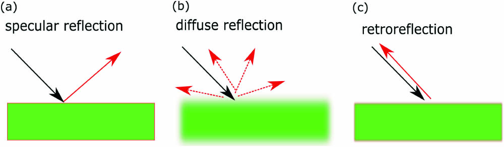
Fig. 1. Different types of reflection: (a) specular reflection, (b) diffuse reflection, and (c) retro-reflection.

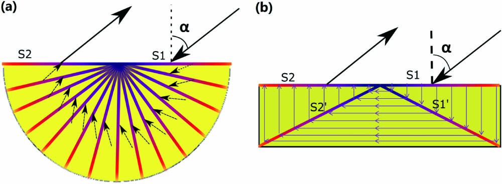
Fig. 2. Schematic diagram using OST to design a retro-reflector. To see the one-to-one corresponding relationship in equivalent surfaces clearly, we use the gradient color to mark each equivalent surface. (a) A half-cylindrical retro-reflector: S1 and S2 are linked by ONMs with axes along the tangential direction. The distribution of the points on S1 and S2 is reversed by 180 deg, and, hence, the output beam is the retro-reflection of the incident beam. (b) A flat planar retro-reflector: ONM with main axis (the purple arrow) along the x direction links S1’ and S2’. ONMs with main axis (the purple arrow) along the y direction link S1 and S2 with S1’ and S2’, respectively. The directions of purple arrows indicate the directions of the electric field projection during the one-to-one transfer procedure. S1, S2, S1’, and S2’ are all equivalent surfaces. The orientations of corresponding points on S1 and S2 (gradient colored) are reversed by 180 deg.

Fig. 3. 2D numerical simulation results for the TE polarization wave case. We plot the absolute value of the normalized electric field distribution. The incident wave is a Gaussian beam with waist radius w0=3λ0. From (a) to (h), the incident angles change from 0 deg to 70 deg.

Fig. 4. 2D numerical simulation results for the thin planar retro-reflector as the incident angle changes from (a) 0 deg to (h) 70 deg. The height and width of the planar retro-reflector are 2λ0 and 12λ0, respectively. The incident wave is a Gaussian beam with waist radius w0=3λ0.

Fig. 5. 2D numerical simulation results for the TE polarization case: we plot the absolute value of the normalized electric field distribution. The white regions are filled by ONMs of various shapes, whose main axis directions are indicated by black arrows. The incident wave is a Gaussian beam with waist radius w0=3λ0. The incident angle is 45 deg in all cases except (d). The geometric shapes of the retro-reflectors are (a) an isosceles triangle, (b) a flat triangle, (c), (d) irregular surfaces, and (e) an array of isosceles triangles. Note that the input and the output surfaces can be irregular surfaces as long as they are complementary, which ensures that the phase fronts of the input and output beams are parallel. The input and output surfaces are no longer symmetric, so we simulate 45 deg incidence in (c) and −45deg incidence in (d). (e) An array of isosceles triangular retro-reflectors in (a). The retro-reflector can be very thin, e.g., 2/3λ0 in (f).

Fig. 6. (a) Efficiency of the planar retro-reflector as incident angle changes. (b) Efficiency of the planar retro-reflector as the height changes.

Fig. 7. Realization of the retro-reflector. (a) Basic diagram using micro-channels. (b) 2D numerical simulation results for the TM polarization wave case with an incident angle of 40 deg. (c) Efficiency of the retro-reflector with respect to different incident angles.