Fig. 1. Assembly of the HTSC-sabot + target, or HTSC-projectile (not to scale): (a) 1 – HTSC-housing, 2 – polymer insert with a target nest on its top, 3 – MgB₂ driving coils, 4 – cryogenic target; (b) 5 – mock-up of the HTSC-housing made from superconducting ceramics, ρ = 4 g/cm^3[4,5], 6 – hole for the polymer insert; (c) 7 – target shell, 8 – solid fuel layer, 9 – vapor fuel.

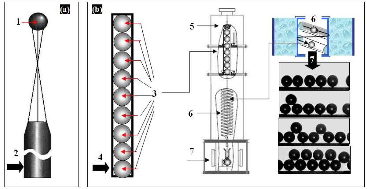
Fig. 2. Comparative efficiency chart of two principally different approaches: (a) traditional (target mounted onto the holder, or one-of-a-kind technique for today’s ICF experiments); (b) free-standing targets, or FST approach, for mass target fabrication under high repetition rate conditions.

Fig. 3. The HTSC-sabots used in the experiments: (a) Sabot #1 (mass is 1.25 g); (b) Sabot #1 with liquid nitrogen inside in the round PMG-1; (c) Sabot #1 levitation with a load capacity of three cylindrical surrogate targets (1.1 g each) in the round PMG-2; (d): Sabot #2 (mass is 1 g) with a polymer foam inside (shown on the right); (e) Sabot #2 acceleration in the inclined linear PMG.

Fig. 4. Repulsion and attraction forces produced by interaction in an HTSC sample: 1 – a piece of YBCO ceramics with dimensions of 1.6 mm × 1.6 mm × 2.2 mm and a mass of 24 mg; 2 – PMG system. The HTSC sample can be suspended above the magnet (a), in the center of it (b) and below the magnet (c).

Fig. 5. Quantum locking as a promising method for target assembly, known as ‘hohlraum’ targets: (a) PS shell (1) with a deposited YCBO-layer at T ~ 80 K, 2 – magnetic holder (NdFeB disk with OD = 15 mm, ID = 6 mm, d = 5 mm plus iron insert with OD = 6 mm, d = 5 mm), 3 – transport belt for magnetic holders placement; (b) holder spacing on the moving belt; (c) cylindrical container mounted onto the holder.

Fig. 6. Schematic diagram of the magnetic track construction: (a) N-S-N elementary block; (b) linear N-S-N magnets arranged in three rows forming a linear track (figure taken from Ref. [11]).

Fig. 7. POP experiments for testing a one-stage linear accelerator: (a) general view of the PMG with only one gap at a length of 24 cm (1 – field coil, 2 – HTSC-sabot (300 K), 3 – gap between the magnets covered in the middle with an iron collector (4), 5 – iron base, 6 – permanent magnets); (b) Sabot #1 at the end of the magnetic track; (c) Sabot #1 during acceleration in the middle of the magnetic track, where the load capacity is six spherical polymer shells of about 0.6 mg each (tandem sabot); (d)–(f) freeze frames of the video recording of Sabot #2 acceleration (view from above).

Fig. 8. Freeze frames of a Sabot #1 jump under the electromagnetic pulse action (B = 0.33 T, τ = 1 ms): (a) before the electromagnetic pulse, liquid nitrogen is poured into Sabot #1, where the observation time (frames a1–a4) is approximately 1 s; (b) initially the coil and Sabot #1 with a load capacity (copper plate inside it) were cooled with liquid nitrogen, and then an electromagnetic pulse was applied to the coil.

Fig. 9. Experimental illustration of the characteristics of the HTSC-PMG maglev linear system: (a) schematic diagram, 1 – field coil, 2 – HTSC-sabot, 3 – PMG system, 4 – magnetic brake (if it is required by the experimental conditions, the system can have left- and right-hand brakes, or one of them, or none); (b) an option of the brake placement in the PMG system; (c) no co-linearity between elements 1 and 2; (d) and (e) collinear element arrangement; (f)–(h) oscillations of Sabot #1 between two brakes under mechanical drive pulse.

Fig. 10. Acceleration length L_a for two values of the HTSC-sabot velocity: 200 and 400 m/s.

Fig. 11. A round PMG system to provide a stable cyclic motion of the HTSC-sabot about the Z-axis: (a) and (b) PMG system design; (c) overview of the ring magnet placed in the iron pot; (d) magnetic field mapping on the ring magnet surface.

Fig. 12. The z-component of the magnetic field (B_z) versus radius (r) above the round PMG at various heights: blue – 1 mm, violet – 4 mm, aquamarine – 7 mm, red – 10 mm, green – 11 mm and black – 16.5 mm. Between 1 and 7 mm above the track, the gradient is still very strong to control the HTSC-sabot trajectory.

Fig. 13. Quantum locking based on the flux pinning effect makes the HTSC-sabot orientation fixed in space so that it will not re-orient itself without any external action (the HTSC-sabot temperature is ~ 80 K).

Fig. 14. Freeze frames of the Sabot #2 rotation along a fixed trajectory (T ~ 80 K): (a) and (b) near the internal PMG border (the levitation height is 6 mm, the average HTSC-sabot velocity is 0.15 m/s); (c)–(e) in the external PMG border (the levitation height is 3 mm, the average HTSC-sabot velocity is 0.8 m/s).

Fig. 15. Freeze frames of the rotation movement of Sabot #1 along a changing trajectory (T ~ 80 K): (a) starting from the PMG middle (frame 1), Sabot #1 gradually picks up its velocity and shifts due to the centrifugal force to the outer PMG border (frame 5); (b) frames 6–8 correspond to the last few turns, and then Sabot #1 stalls from the trajectory when its velocity becomes equal to 1.48 m/s.

Fig. 16. The round PMG system with magnetic propulsion (T ~ 80 K): 1 – field coil (the drive pulse is generated in the sabot position corresponding to frame 1), 2 – Sabot #1, 3 – NdFeB ring magnet.

Fig. 17. An option of the cyclic HTSC-maglev accelerator for target delivery at the laser focus: 1 – HTSC-projectile (HTSC-sabot + target), 2 – TLS, 3 – start (input) coil, 4 – field coils, 5 – magnetic rail, 6 – brake (output) coil, 7 – used HTSC-sabot, 8 – SCS, 9 – target after separation from the HTSC-sabot, 10 – tracking system; 11 – to the reaction chamber. In this scheme, the start (3) and brake (6) coils can play the role of the field coils (4), which simplifies the accelerator design. The HTSC-sabot (7) can be reused again and again in the target delivery system.

Fig. 18. An oval-shaped PMG with a length of 22 cm and a width of 9.5 cm was build up from four individual tracks to alternate acceleration (track 1) and rotary functions (track 2), having four gaps between them (3): (a) general view of the PMG system; (b) magnetic field mapping by MFV film; (c) Sabot #1 (with liquid nitrogen inside, T ~ 80 K) at the output of the round track.

Fig. 19. First experiments with an oval-shaped PMG without any gaps (‘one-piece’ design or non-composite magnet): (a) stable levitation of Sabot #2 (T ~ 80 K, HTSC-sabot axis along the track); (b) magnetic field mapping by MFV film; (c) stable levitation of Sabot #1 (T ~ 80 K, HTSC-sabot axis across the track).

Fig. 20. The magnetic force field K_r versus track radius for different injection velocities: 1 − η = 1.0 × 10³ g/cm³, V_inj = 200 m/s; 2 − η = 2.5 × 10 ³g/cm³, V_inj = 100 m/s; 3 − η = 4.5 × 10³ g/cm³, V_inj = 50 m/s.

Table 1. Target acceleration requirements for ICF.

Table 2. Field coil working parameters used in the HTSC-sabot acceleration experiments.

Table 3. MSL accelerator parameters in the case of V_inj = 200 m/s (values are specified for driving coils from MgB₂ at T_S = 20 K).