The past years have seen a great success of deep neural network (DNN), especially when it comes to using the CNNs for typical computer vision tasks, such as image classification, pattern recognition, object detection and so forth. However, one commonly ignored fact is that, in the most cases, such remarkable performance is obtained at the cost of huge consumption of computing resources. With the topology of neural network going deeper, the case could be even worse. Take the CNN model from ILSVRC^[1] as an example, compared to AlexNet^[2], ResNet152^[3] improved the top-5 classification accuracy by ~11.7%, while the running FLOPs soared to more than 10x. As a result, the training and inference of the state-of-the-art models suffered from large resource requirement and poor energy efficiency. Moreover, the training phase can last for weeks because of the sophisticated model architecture and the time-consuming floating-point arithmetic operations. The floating-point operations are also unfriendly to the hardware accelerations on ASIC or FPGA. To address this problem, model compression has been proposed, which helps to drastically reduce the arithmetic complexity and thus alleviate the computing workload.

Recent works on model compression basically lie in two categories: pruning and quantization. Pruning means that there is sufficient redundancy in common DCNN models^[4], hence a number of weights can be eliminated from neuron connection^{[5, 6]}. However, since pruning introduces some irregular connections between neurons, the dataflow in the feed-forward pass has to be rearranged in order to organize the whole process correctly and efficiently, which usually requires dedicated hardware design on ASIC or FPGA platform.

As for quantization, instead of using single-precision floating-point format, it represents weights (W), activations (A) and gradients (G) with limited numerical bit-width. In this way, quantized networks are enabled to replace the time-consuming floating-point processing elements with integer-based arithmetic units, therefore the amount of operations can be dramatically reduced. In the meanwhile, as a byproduct of limited bit-width representation, the demand for storage will shrink greatly, which is quite an appealing feature since the size of parameters in recent networks can be as large as ~10 M. Based on the way of generating quantized neural network parameters, related works can be further classified into two types: quantizing with pre-trained networks and training from scratch^[7]. It is obvious that the former ones still rely on high-precision networks, and they are mainly targeting the inference phase in deployment. To equip edge devices with complete ability to perform both training and inference, the latter ones, also known as fully quantized networks, deserve more efforts.

In the era of IoT, deep learning techniques have been expected to be applied in wide industrial scenarios, yet high power demand and poor energy efficiency remain main barriers for its popularization. Quantized neural networks provide a promising solution to solve the problem. In this work, we aim to develop a quantized training flow with most of the parameters quantized to 8 bits and train the network from scratch under a very limited classification accuracy degradation. Our contributions can be summarized as follows:

(1) We achieve quantized neural networks for training from scratch with limited classification accuracy degradation for CNN.

(2) We evaluate the quantization scheme on a RNN model and obtain very similar outcome to its single-precision counterpart.

(3) We develop a FPGA prototype to validate the feasibility of the proposed scheme and evaluate the resource usage.

A lot of experiments are performed on prevalent state-of-the-art DNNs and datasets. It is demonstrated that we achieve 0.12% top-1 accuracy drop for ResNet-20 on Cifar-10 dataset. We achieve 0.42% top-1 accuracy drop for AlexNet. We achieve 1.31%, 1.92% top-1 accuracy drop for ResNet-50 and Inception V3 models, respectively. As for the prototype, the synthesis results show that we reduce the DSP usage by ×106, we reduce the BRAM usage by ×1.97, we reduce the FF usage by ×6.23, we reduce the LUT usage by ×2.9. Besides, for translation models, we achieve an 8-bit GNMT model with 24.05 BLEU, which is close to 24.46 achieved by a single-precision model.

Among all quantization methods, the basic procedure to quantize a given vector (or tensor) x is to perform a transform function upon it, which is called the quantization function. Assume that the original vector to be quantized is represented in 32-bit floating-point format, and our ultimate goal is to replace it with 8-bit fixed-point representation. In this work, we choose the dynamic fixed-point (DFP) as our quantization method.

In this section, firstly, the details of the DFP quantization algorithm are provided, including the basic principles of updating scale integers and the bit-width settings in the MAC operations and back propagation datapath. Secondly, some other typical quantization methods are introduced and analyzed to form a comparison to DFP. The strengths and weaknesses of different quantization methods are pointed out respectively.

Among all types of layers in DCNN, convolution layer and fully-connected layer account for more than 90% of the computing time^[8]. Therefore, quantizing feature maps and parameters in these layers provides the most benefits. In order to quantize the tensors from 32-bit to 8-bit and keep the representation precision to the largest extent, we use the dynamic fixed-point (DFP) representation^[9]. The DFP format is based on fixed-point representation, while the scale factor is dynamically adjusted. Concretely, each element of a tensor in DFP format is represented by an 8-bit signed integer. Meanwhile, the tensor also comes with a signed integer e representing its scale. For each entry of this tensor with value x (in 8-bit signed integer), the actual value it represents is thus . The scale integer e is updated constantly during the training process.

Given the scale e, the original tensor in 32-bit floating-point format is quantized to 8-bit DFP by approximating each floating-point number to the closest representable DFP number, i.e. , , , , , . The quantization method is deterministic. We also used stochastic quantization (rounding) for the representation of gradients, and the details are covered in Section 3.

The scale integer is chosen such that the numerical resolution is as high as possible, without having overflow. For implementation, is chosen to be a fixed number at the start of training. For every training batch, is incremented if there is an overflow in quantization, and is decremented if doing so does not lead to an overflow. According to Ref. [9], the DFP quantization scheme can be summarized as in Algorithm 1:

Algorithm 1 Dynamic fixed-point

Inputs: tensor x to be quantized, scale integer e_i w.r.t x in the ith iteration, overflow rate r_max

Output: updated scale integer in the iteration

1: compute the overflow rate for tensor

2: compute the overflow rate for tensor

3: if then

4:

5: else if then

6:

7: else

8:

9: end if

To be more concrete, we set the overflow rate . Given the input tensor x, we firstly re-scale it to another tensor through a mapping function :

$ \widetilde{x} = f(x) = x \; /\; 2^e. $ ()

Then, with the quantization bit-width n, let S denote the interval , the overflow rate of input tensor x can be determined as follows:

$ {r_x} = \left\{ {\begin{array}{*{20}{l}} 1, & {{\rm{if}}\;{\rm{any}}\;{\rm{entry}}\;{\rm{of}}\;\widetilde x\;{\rm{falls}}\;{\rm{out}}\;{\rm{of}}\;{\rm{the}}\;{\rm{interval}}\;S,} \\ 0, & {{\rm{if}}\;{\rm{all}}\;{\rm{entries}}\;{\rm{of}}\;\widetilde x\;{\rm{lie}}\;{\rm{in}}\;{\rm{the}}\;{\rm{interval}}\;S.} \end{array}} \right.$ ()

Similarly, one can compute the overflow rate of 2x. In this way, DFP guarantees that the scale integer is neither too big nor too small with respect to the input tensor x. Eventually, when the training is done, all scale integers will be fixed for the inference stage.

Both convolution and fully-connected layers are based on the multiply-and-accumulate (MAC) operation. Although designing an algorithm that performs both multiplication and accumulation in 8-bit is certainly beneficial, we choose to perform 8-bit multiplication and 32-bit floating-point accumulation. Since quantized networks mainly aim to reduce the consumption of computing resources, the priority lies in the optimization of 32-bit multiplications, while the overhead of 32-bit addition is significantly smaller and thus acceptable. In this way, useful information can be preserved with a minimized computation workload to enable effective network learning.

In terms of the back-propagation data path, all parameters are kept in 32-bit floating-point for gradient descent and update. However, following the spirit of minimizing computation complexity, we ensure that the operands of tensor multiplication are represented in 8-bit DFP. For example, considering the gradient with respect to the weight in a convolution layer, which can be generated by the following formula^[10]:

$ \frac{\partial L}{\partial w^{l}_{jk}} = a^{l-1}_{k}\delta^{l}_{j}. $ ()

Here, the activation and the error are guaranteed to be 8-bit DFP such that the multiplication operation can benefit from the efficient integer operation. As for the gradient w.r.t. the weight , it is represented in single precision floating-point and will be directly used to update the corresponding weight. Since the vanishing of the gradient is particularly severe in fully quantized networks, representing them in 32-bit floating-point format is necessary. Nevertheless, the cost is almost negligible.

To sum up, DFP algorithm is hardware-friendly because the quantized tensors can be represented with pure integers, which serve as the operands in MAC operations, while the quantization process itself introduces no complex floating-point operations like multiplications or divisions.

Apart from DFP, various quantization methods have been emerging over these years. In some quantization methods, the numerical resolution between adjacent symbols of the codebook is fixed, whilst in some others, it varies according to the mapping function. Accordingly, a method can be categorized as either linear quantization or non-linear quantization.

The linear quantization is a method where the resolution is fixed under the input tensor x. Intuitively, to approximate x with a finite codebook, the discrete values can be uniformly appointed over the range between its smallest and biggest entries. This can be expressed as the following formula^{[11, 12]}:

$ Q(x) = {\rm{min}}(x) + {{step}}\times {\rm{Round}}(\frac{x-{\rm{min}}(x)}{{{step}}}). $ ()

Here, Round() is the rounding function, which will be explained in Section 3. step is the fixed interval value between adjacent discrete values and is computed given the input tensor x and the quantization bit-width n:

$ {{step}} = \frac{{\rm{min}}(x)-{\rm{min}}(x)}{2^{n}-1}. $ ()

Apparently, such a basic linear quantization method enables to fit the value of input tensor automatically without the extra concern about dealing with an overflow. However, the method is inevitably sensitive to any outlier in the input tensor. For instance, if the biggest entry deviates from the second biggest entry too much, the above-mentioned method will suffer from severe quantization noise.

In contrast, the interval values between adjacent discrete symbols are different in non-linear methods. Logarithmic quantization^[13] is one of the common non-linear algorithms. The corresponding transformation function is:

$\begin{array}{l} Q(x) = \left\{ \begin{align} & 0, & & {\rm{if}}\;{\rm{scalar}} \; x = 0, \\ & 2^{\widehat{x}}\cdot {\rm{sgn}}(x), & & {\rm{if}}\;{\rm{scalar}} \; x\ne0. \\ \end{align} \right. \end{array} $ ()

Here, the quantization function performs element-wise operations. That is, for each entry of the input tensor x, the function treat it respectively. The sign function is responsible for determining the sign of scalar x, and the output is either 1 or –1. In the end, a quantized matrix is generated. The calculation of is where the logarithmic arithmetic takes place, namely:

$ \widehat{x} = {\rm{Round}}({\rm{log}}_{2}(|x|)). $ ()

The ultimate goal of logarithmic quantization is to replace the complicated MAC operation with simple bit-shift, which is extremely cheap in digital circuit design. Undoubtedly, logarithmic quantization helps to speed up the MAC operations greatly, however, according to the experimental results reported by Ref. [13], the drop of classification accuracy is typically greater than other methods. Moreover, the logarithmic arithmetic itself is intrinsically not hardware-friendly, which sets a barrier for deployment in embedded systems.

Other non-linear quantization methods introduce different ways to establish the mapping from the symbols of the "codebook" to real values. Some use explicit functions, like the tanh function that is used to quantize weights in DoReFa-Net^[14], while others provide a set of discrete values to better match the statistical features of parameters. Take Ref. [15] as an example, where Cai et al. investigate the distribution of network activations in order to devise an half-wave Gaussian quantizer, which is used to approximate activations and can alleviate the gradient mismatch in back-propagation.

In general, although non-linear methods have their unique advantages, the incurred non-linear operations are too expensive in most cases. Under a fixed quantization bit-width, linear methods could bring a better trade-off between the performance and hardware resources cost.

Obviously, with the reduction of bit-width, the numerical resolution inevitably goes down to some extent. In fact, the quantization function can be conceptually decomposed into two separate steps. In the first step, as is aforementioned in Section 2, the vector x is mapped to a proper interval via scaling :

$ f: x \rightarrow \widetilde{x}. $ ()

Following the notation of the Number Theory, we divide the scaled tensor into its integer part and its fraction part , such that:

$ \widetilde{x} = \left\lfloor {\widetilde{x}} \right\rfloor + \{\widetilde{x}\}. $ ()

Actually, the integer part corresponds to the 8-bit fixed-point representation without a decimal point, while the fraction part will be discarded and that is where the precision loss exists.

After re-scaling the original tensor to , the second step is to approximate the fraction part to 0 or 1. Finally, the rounded bit (0 or 1) is added back to the integer part to form the ultimate 8-bit integer. We define the overall process of generating the low bit-width integer from re-scaled tensor as the Rounding function.

Apparently, the most intuitive way to approximate a fraction value is nearest rounding (NR), which means the outcome will be the closest representable discrete value:

$ {\rm{NR}}(x) = \left\{ \begin{align} & \left\lfloor { x } \right\rfloor, & {\rm{if}} \; 0 \leqslant \{ x \} \leqslant \frac{1}{2}, \\ & \left\lfloor { x } \right\rfloor + 1, & {\rm{if}} \; \frac{1}{2} \lt \{ x \} \lt 1. \\ \end{align} \right. $ ()

However, nearest rounding may incur severe quantization noise, which can be the major factor influencing the performance of quantized networks. To address this issue, Stochastic Rounding (SR)^[16] was proposed. Unlike nearest rounding, stochastic rounding is not a deterministic rounding mode, which means the result can be different over multiple attempts. Specifically, it is decided by both input value and a computed probability:

$ {\rm{SR}}(x) = \left\{ \begin{align} & \left\lfloor { x } \right\rfloor, & & \text{w.p}. \; 1-\{ x \} ,\\ & \left\lfloor { x } \right\rfloor + 1, & & {\rm{w.p.}} \; \{ x \} .\\ \end{align} \right. $ ()

Generally, the target of rounding functions is to convert the scaled vector to an integer that can be represented with limited number of bits. Let n denote the quantization bit-width and assume that we adopt signed integers, then the range set of rounding functions should be , , , , , . Hence regardless of the rounding function used, outlier values need to be coped with through clipping mechanism:

$ {\rm{Round}}(x) = \left\{ \begin{align} & -2^{n-1}, & & {\rm{if}} \; x \leqslant -2^{n-1} ,\\ & 2^{n-1}-1, & & {\rm{if}} \; x \geqslant 2^{n-1}-1, \\ & {\rm{NR}}(x)\; {\rm {or}}\; {\rm{SR}}(x) , & & {\rm{otherwise}}. \end{align} \right. $ ()

Despite the fact that SR is not hard to understand, to implement it could be another problem, as a 1-bit random number generator with a floating-point possibility value will be needed. Needless to say, such a module would be a huge challenge for hardware designers, especially for those who wish to get rid of floating-point arithmetic. However, if we think about the SR carefully, the randomness within rounding possibilities can be exploited in another equivalent way. Consider a random value that obeys the uniform distribution:

$ \varepsilon \sim U(0,1). $ ()

Then the SR function can be equivalently expressed as^[17]:

$ {\rm{SR}}(x) = \left\lfloor { x+\varepsilon } \right\rfloor. $ ()

It should be noted that the equivalence can be easily proved statistically. Consider the value of in a random experiment, it is obvious that:

$ \begin{array}{l} \varepsilon \in \left\{ {\begin{array}{*{20}{l}} {[0,1 - \{ x\} ),} & {{\rm{w}}.{\rm{p}}.\;1 - \{ x\} ,}\\ {[1 - \{ x\} ,1),} & {{\rm{w}}.{\rm{p}}.\;\{ x\} ,} \end{array}} \right.\;\; {\rm{such}}\;{\rm{that}} \\ \;\;x + \varepsilon \in \left\{ {\begin{array}{*{20}{l}} {[x,1 + \left\lfloor x \right\rfloor ),} & {{\rm{w}}.{\rm{p}}.\;1 - \{ x\} ,}\\ {[1 + \left\lfloor x \right\rfloor ,1 + x),} & {{\rm{w}}.{\rm{p}}.\;\{ x\} .} \end{array}} \right. \end{array}$ ()

In this way, the SR function can be further expressed as following:

$ {\rm{SR}}(x) = \left\lfloor { x+\varepsilon } \right\rfloor = \left\{ \begin{align} & \left\lfloor { x } \right\rfloor, & & {\rm{w.p.}} \; 1-\{ x \}, \\ & \left\lfloor { x } \right\rfloor + 1 , & & {\rm{w.p.}} \; \{ x \} .\\ \end{align} \right. $ ()

This is exactly the same as the original definition. To some degree, the merit of adopting additive uniform noise lies in that probability is exploited in an implicit way. Instead of the complicated 1-bit random generator with an arbitrary possibility ranging from 0 to 1, an ordinary uniform random number generator will be enough to implement the stochastic feature, which can be realized by utilizing some existing hardware libraries.

Recently, stochastic rounding has been widely accepted as an effective strategy to acquire better performance in quantized DCNNs^{[13, 17, 18]}. Yet there have been scant works trying to reveal the reason behind the success of SR. One noticeable progress^[7] is that theoretically analyzed the convergence of SR, along with its limitations^[7]. In this work, we try to explain from an empirical perspective and put our emphasis on the necessity to replace NR with SR.

As is claimed in DoReFa-Net^[14], to achieve better performance, gradients need to be allocated with wider bit-width and should be stochastically quantized. Moreover, it can be summarized from our experiments that applying SR to the quantization of gradients actually helps to stabilize the gradient descent process. As a result, the initial learning rate can be set to a bigger value to avoid the local optimum phenomenon.

To better understand the mechanism, consider a toy example where is a random variable that obeys a normal distribution:

$ X \sim N(0,3^2). $ ()

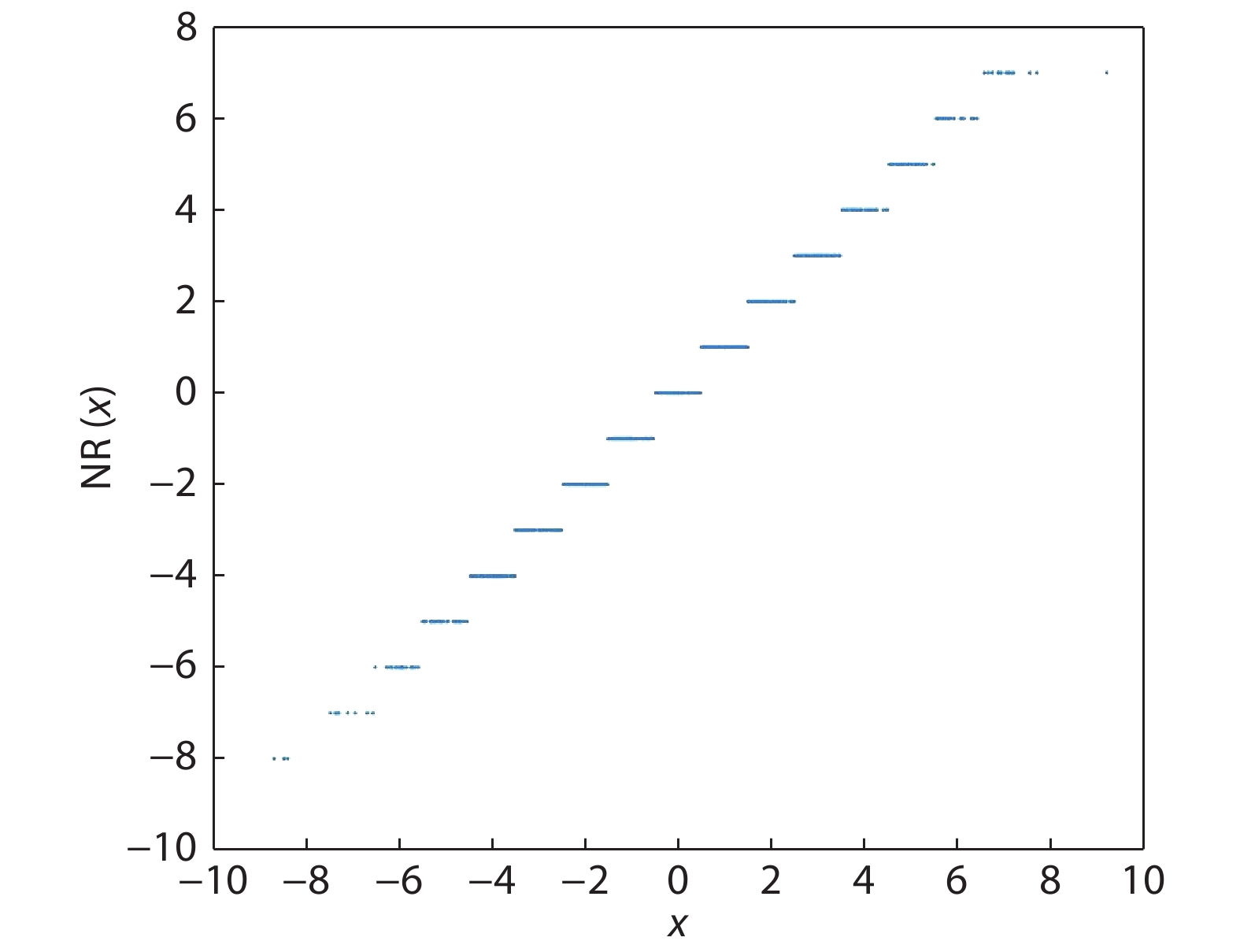
We take X as an example to simulate the scaled parameters within the quantized DCNN. Assume that the quantization bit-width is 4, so we have 16 discrete outcome in total. During simulation, we generate 1000 value according to the normal distribution which are then taken as the input of both NR and SR. Figs. 1 and 2 summarize the results of simulation.

As is depicted in Figs. 1 and 2, SR enables an input scalar to have multiple corresponding symbols in the codebook, which essentially enhances the flexibility of quantization. Unlike NR which deterministically generates the outcome, SR randomly determines whether to round up or down. Most importantly, it should be noted that SR helps to compensate the vanished values, which is particularly significant in gradient quantization. Consider an item of a gradient tensor whose value lies in the interval ( , 0.5], if we apply NR to it, the outcome will be undoubtedly 0, which means the value will simply vanish and will have no influence on the update of parameters to be learned. However, SR will make a difference, since apart from 0, the outcome can be either –1 or 1, which will ultimately contribute to the learning phase. It should be noted that, in fully quantized networks, the noise effect incurred by quantization could be accumulated layer by layer, and lead to an unacceptable drop of classification accuracy on the whole. Hence, preventing small values from vanishing is extremely important in the training process.

To further evaluate the influence of different rounding functions, we carry out experiments on AlexNet and ResNet18 to compare the classification accuracy with NR and SR, respectively. In order to provide a fair comparison, we guarantee that all the training hyperparameters are the same and the only difference is the rounding function. The corresponding results are summarized in Table 1.

As is shown in Table 1, rounding function can affect the classification accuracy greatly in AlexNet, which is consistent with our analysis and simulation. We also notice that rounding function has a relatively slight impact on ResNet-18, which is probably the consequence of the residual block that enhances the gradient value in back propagation.

In this section, the proposed fully quantized network is evaluated on several prevalent CNN models and datasets. Furthermore, we have performed evaluations on some translation models to study the feasibility of limited precision training on other tasks. Our implementation is released in PyTorch.

With 50 000 training images from 10 categories and 10 000 validation images, CIFAR-10 is chosen as a small-size dataset to test the performance of quantized models. We quantize all parameters (W, A, G) using 8-bit DFP in both forward pass and backward pass. All parameters are rounded with NR, except for the gradients exploiting SR. A single NVIDIA GeForce GTX 1080Ti GPU card is used for execution and the batch size is 128. The initial learning rate is 0.1, then decay in cosine annealing manner over 150 epochs. We adopt SGD optimizer with the momentum value being 0.9. We use weight decay as well and the value is set to . Both ResNet-20 network and ResNet-56 network are tested. Table 2 shows their top-1 accuracy of full-precision and low-precision networks, respectively.

It can be concluded that fully quantized networks can achieve almost identical classification accuracy to its single-precision counterparts, even in deep networks like ResNet-56. We believe that such results mainly benefit from the small size of CIFAR-10 dataset and the corresponding limited number of classification categories. To test the stability and performance of fully quantized networks, the evaluation on a larger dataset would be more effective.

ImageNet (ILSVRC2012) is another benchmark chosen in our evaluations, which has ~1.28 × 10⁶ training images from 1000 categories and 50 000 validation images. Similarly, we quantize all parameters (W, A, G) using 8-bit DFP in both forward pass and backward pass. All parameters are rounded with NR except for the gradients, which adopt SR. Since images in ImageNet dataset belong to as many as 1000 categories, the average predicted probabilities will be two orders of magnitude smaller than those in CIFAR-10. To cope with this issue, we set the quantization bit-width in the last fully-connected layer to 16-bit, such that the codebook is expanded significantly and the extremely small values can be approximated more precisely.

A group of 8 NVIDIA Tesla V100 GPU cards are used for execution and the batch size is 256 ( ). The learning rate of full-precision network starts at 0.1, while we found the best initial learning rate of low-precision model that can converge is 0.05. The decay of learning rate still follows cosine annealing manner over 120 epochs. We adopt SGD optimizer with the momentum value being 0.9. We use weight decay as well and the value is set to 1 × 10^–4. Several popular networks are tested, namely AlexNet, ResNet-18, ResNet-50 and Inception V3. Table 3 shows their top-1 accuracy of full-precision and low-precision networks, respectively. (Note: The 32-bit accuracy is directly obtained from our PyTorch implementation under the same hyperparameters as 8-bit model, which is slightly lower than the corresponding accuracy provided in the official documents)

As can be observed from Table 3, fully quantized networks targeting ImageNet suffer from greater accuracy degradation. With the topology going deeper, the degradation could be even larger. Unfortunately, there are very few related works to compare with, since many works on low-precision networks are merely quantized on the inference phase. As for fully-quantized networks, some use very different bit-width for W, A and G.

We noticed that in DoReFa networks, there is one instance of AlexNet where W, A and G are all quantized with 8-bit and the ultimate accuracy drop is 2.9%. In our experiment, we achieve only 0.42% accuracy drop. Please note that in terms of full-precision AlexNet, our accuracy is slightly lower than that given by DoReFa-Net. The resaon is that our network is consistent with the official implementation from PyTorch library^[19], which does not include the batch norm layer. Even so, given the fact that DoReFa requires the first input layer and the last layer to stay completely unquantized, this is actually a remarkable improvement. We owe the success to DFP quantization algorithm and the exploration of optimal training hyperparameters.

To be more specific, DoReFa-Net adopted linear quantization for the gradient, which is similar to the aforementioned linear method. In practice, such method can lead to significant deviation caused by some outliers, especially when it comes to the gradient. Consequently, the quantized gradient makes it more difficult to converge, which leads to higher drop in classification accuracy.

To demonstrate that our quantized training framework can be applied to deep networks other than CNNs, we implement a recurrent neural network (RNN) using DFP. We consider a GNMT model^[20] for machine translation based on the open source implementation of NVIDIA^[21]. The network contains a 4-layer encoder and a 4-layer decoder with attention modules^[22]. The network is trained and evaluated using an English-German translation dataset, and the evaluation metric is the BLEU score^[23]. The quantized GNMT model uses 8-bit DFP except the last layer of the decoder, which uses 16-bit DFP. The training strategies are the same as Ref. [16]. Our experiment showed that the 8-bit GNMT model achieves a BLEU score of 24.05 on the test set, which is closed to 24.46 achieved by a full precision model.

According to the proposed quantization algorithm, we implement the FPGA prototype using Vivado HLS. The design consists of a central controller and several modules corresponding to different layers. We adopt the layers in Caffe framework. There are totally eight types of layers, namely convolution, batch normalization, scale, relu, pooling, element-wise (eletwise), fully-connected, and softmax. For each type of layer, different modules handle the forward pass, backward pass, weight update and bias update, etc. The central controller coordinates the execution of all the modules in a layer-by-layer fashion. Fig. 3 shows all the modules we have implemented to support the popular neural networks. Totally 21 modules are implemented. Each kind of layer holds a forward module and a backward module for activation and gradient calculation in the forward pass and backward pass, respectively. Only convolution, fully-connected and scale layers have the additional weight and bias update modules since they are equipped with weights and bias. Only one module handles the softmax related calculation. The softmax module takes the activation from its preceding layer as input, calculates the gradients for back propagation according to the ground-truth labels, and generates the softmax outputs.

The whole design structure is shown in Fig. 4. The instruction table defines the information for execution of each layer. During training, the central controller fetches the instruction for one layer each time and activates the corresponding modules. After the modules complete execution, the central controller fetches the instruction of the next layer, and coordinates the execution in such a layer-by-layer fashion. In the forward pass, the central controller fetches the instructions from smaller index to larger index, where the smaller index indicates the layer close to the beginning of the neural network. After the forward pass, the central controller will start the backward pass to fetch the instructions from larger index to smaller index, so that the layers can be executed reversely for back propagation. In the forward pass, the forward module is activated for the layer while in the backward pass, the backward module, weight update module and bias update module will be activated one by one. At a specific time spot, only one module is running in our design. During the execution of each module, the module will get the address offset for its related data from the central controller according to the corresponding instruction. The module loads and stores its related data, such as the activations, gradients, weights, bias, etc., from and to the off-chip DDR through the load and store interface during execution.

The instruction table is stored as an array to define the neural network structure, where each row of the array is one instruction and corresponds to one layer in the neural network. The content of the instruction indicates the specification of the layer. Each instruction specification contains the information for the type of the layer, the parameters of the layer including channel numbers, padding size, stride size, kernel size, etc., the top and bottom layer ID connected to this layer, etc. Through the top and bottom layer specification, the connections in the neural network can be defined. All the related data for each layer including the activations in the forward pass, the gradient in the backward pass, the weights and the biases are stored in the off-chip DDR with specific address offsets. The address offsets are also contained in the instruction table, so that the corresponding module can access the related data in the DDR. For the layers with direct connections, the address offset of their input and output data are the same, so that the data communications between layers are achieved in a shared memory way. We develop a compiler to compile the network specification from an Caffe prototxt file into the instruction table. A Caffe prototxt file defines the network structure with specified layers and their connection relationships. During the training, when the central controller activates each module, it will also set the required parameters for the module from the instructions, such as channel numbers, padding size, stride size, kernel size, etc.

According to our algorithm, we keep each weight and bias as two versions, floating-point and 8-bit dynamic fixed point. Floating-point version is used to be updated in the backward pass for the accuracy, then it is quantized to 8-bit for all the other computing with increased computing efficiency. The activations in forward pass and gradients in backward pass are represented in 8-bit dynamic fixed point for most layers, which is strictly in consistency with our PyTorch implementation. Therefore, in the forward pass and backward pass module, the inputs are all 8-bit dynamic fixed point data and the calculation can be simplified to 8-bit operations. Then the results are quantized back to 8-bit dynamic fixed point data as the output from the module. For each weight and bias update module, the gradients and activations used as the calculation input have been already quantized into 8-bit dynamic fixed point in previous forward pass and backward pass executions. These 8-bit data are used to calculate for updating the 32-bit floating point weights and bias. After the execution of weight and bias update modules, the corresponding floating point version weights and biases in the DDR will be updated. Then the corresponding weights and bias in 8-bit dynamic fixed point version will be also updated according to the updated floating point version.

We adopt the SGD optimizer with momentum for update, hence a historical value for momentum should be kept for each weight and bias, which is stored in single precision floating-point for accuracy. Through quantization to 8-bit dynamic fixed point, the multiply-and-add (MAC) operations in convolution, fully-connected and scale layers can be simplified to 8-bit calculation with better efficiency in both speed and resource. To further enhance the computing efficiency, the computation-intensive modules are executed with high parallelism in both batch dimension and output channel dimension. For example, in the forward pass module of convolution, the calculation for several images in the batch are executed simultaneously and the results for multiple number of output channels are executed at the same time. For the softmax and batch normalization layers, due to the complex exponential and square root functions, 32-bit floating point data is required to do both the forward pass and backward pass calculation. Since the activations and gradients are 8-bit, for these two layers, we first convert the 8-bit input back to floating point, do the calculation, and then convert the floating point data as 8-bit dynamic fixed point output.

We explore the parallelism in the module design for computing efficiency. For main computing layers such as convolution, fully connected, scale, relu, etc., we perform the parallel execution in two dimensions, the batch dimension and output channel dimension. At the same time, we calculate for PARA number of output channels and calculate for all the images in the batch. Therefore, the parallelism is PARA × Batch Size is our case. Fig. 5 shows the basic structure for the convolution forward pass module as an example. Each execution unit (EU) is in charge of the calculation for one output channel. Inside each EU, Batch Size number of calculations are performed in parallel. Each EU calculates the output at the same (x,y) position in the image simultaneously, thus they can share the input data with different weights and bias. In this way, we can achieve high parallelism with reduced data load overhead. To support such parallelism and batch calculation, we organize the activations and gradients in [height, width, channel, batch] fashion to provide the data loading and storing with more locality for better efficiency. After the calculation, the output data will be passed to the quantization unit before to DDR. The quantization unit will quantize the 32-bit integer result from the MAC operation back to 8-bit dynamic fixed point. The design concept and overall structure of the other modules are basically the same as this example. For some layers, such as batch normalization and softmax, the quantization unit should be also designed at the input buffer to convert the 8-bit dynamic fixed point back to floating-point first for calculation. For the weight and bias update modules, both quantized output for 8-bit version and non-quantized output for the floating-point version will be sent to the DDR.

The random number generators used in the quantization unit for the stochastic rounding are designed as a 16-bit linear-feedback shift register to generate pseudo random numbers with a given seed. The generator is shown in Fig. 6. The 16 bit data is first set to a seed value. Then each time the 16-bit value does a right-shift operation with the XOR result from four of its bits as the new leftmost bit value. Such a linear-feedback shift register can guarantee good randomness. In our design, different random number generators will get different random seeds. Moreover, at each training iteration, the seeds will be reset as different 16-bit random numbers to the whole design as a parameter, to further ensure the randomness. During the experiments, we have also verified the good randomness of the generated random numbers. The quantization follows the stochastic rounding strategy and dynamic fixed point representation. Since stochastic rounding is only needed in the backward pass, the random number generators are only set in the backward modules. After the main calculation of the module, such as the EU parts in the backward convolution module, the calculated results are sent to the quantization unit in a sequential manner. Each result will go through the stochastic rounding using one random number from a random number generator in the quantization unit. Totally, 7 random number generators are needed, which saves the resource usage and reduces design complexity. However, such a sequential quantization design may affect the whole throughput, which can be further improved in the future work.

The whole FPGA design shows the same functionality as the python code, with the same outputs and training ability. We map the ResNet50 design from the Caffe prototxt file onto Vertix Ultrascale+ XCVU9P FPGA with the clock rate being 200 MHz. The observed peak throughput can be as large as 102 GOPS. The resource usage is as in the Table 4. The parallel degree of this implementation is 16 × 16, which means the parallelism is 16 in the batch dimension and 16 in the output channel dimension. All the modules for different layers are implemented on the FPGA at the same time while only one module is running at one time, therefore the peak throughput is limited. Pipelining among different layers in the layer-fusion style can be considered to further improve the design, although which is quite complicated and beyond the scope of this work. Without quantization, the design cannot achieve the parallelism of 16 × 16 due to the lack of DSPs since all the operations are in floating point with the demand of using DSP. Through quantization using 8-bit dynamic fixed point in our design, the resource usage demand is decreased by a large degree to enable larger parallelism.

In summary, DFP quantization reduces the resource usage significantly. For example, for a convolution layer, our design with quantization reduces the number of DSP usage from 5124 to 48 (by 106x), reduces the BRAM block usage from 162 to 82 (by 1.97x), reduces the FF usage from 466926 to 74933 (by 6.23x), reduces the LUT usage from 412630 to 141828 (by 2.9x). Hence, with quantization, our low bitwidth training scheme can explore more parallelism with limited resource to boost the performance. The current FPGA prototyping is relatively simple without further optimization, since our work mainly focuses on the algorithm level. Further optimization of the hardware implementation are left as future work to further improve the throughput.

In this work, we develop and implement fully quantized DNN with minimum accuracy degradation. We find DFP to be an appropriate quantization method that is both hardware-friendly and well-performed in numerical approximation. Our FPGA based prototype proved that the design works correctly and the training scheme can be mapped to hardware efficiently. The required hardware resource can be dramatically decreased without noticeable drop in performance. However, there is large room to improve the design and hardware implementation in the future works.

Theoretical analysis. In this work, we show the benefits of stochastic rounding over the nearest rounding through simulation and experiments. However, we believe some theoretical analysis regarding the comparison will be more convincing and solid. Similar to Ref. [7], this may include convergence analysis, mathematical modeling, etc.

Quantization methods. As mentioned previously, there are various quantization functions with their respective pros and cons. Despite DFP works fine in our design, it is not certainly to be the optimal method. For example, it is argued that feature maps and parameters to be quantized in networks do not obey symmetrical distribution around zero^[11]. Adaptive methods which can dynamically adjust the mapping function and more sophisticated quantization schemes might become better solutions in the future.

FPGA implementation optimization. Fully quantized low-precision networks are expected to be implemented on embedded systems in the end. In this work, we studied the design methodology of FPGA implementation and designed a simple prototype, while there is still a large room left for optimization. In the future work, deeper pipelining, fusion of layers, and the reduction of SR overhead need to be further explored to significantly improve the throughput of the design.

The research regarding low precision neural networks has been attractive over last several years. BinaryConnect^[24] is thought to be the first attempt to quantize contemporary neural networks, where only weights are binarized. BinaryConnect achieves identical accuracy to full precision networks on CIFAR-10. BNN^[25] further binarize both weights and activations and the evaluation shows little accuracy drop as well. Challenging large dataset and deep architectures with quantized networks was pioneered by XNOR-Net^[26]. However, XNOR-Net find that binarizing activations in addition to weights could introduce an accuracy drop which is as large as 12.4%.

Such results naturally arouse a question: Which kind of parameters (i.e. W, A, G) in neural networks should we allocate more number of bits to prevent severe degradation in accuracy? DoReFa-Net^[13] answers the question and managed to draw a conclusion: The order of required quantization bit-width among parameters is .

In addition, Wage^[27] also targets quantized neural networks for both training and inference, where batch-normalization (BN) is replaced by constant scaling factors to improve regularization. The erasing of BN actually removes a huge obstacle in quantized networks.

In terms of works closely related to stochastic rounding, HALP^[18] takes inspiration from SR to propose a novel low-precision SGD optimizer. Lin and Talathi investigate the difficulties of training low-precision networks and provides more complementary techniques that are orthogonal to SR to combat the instability and improve the training outcome^[28].

In this paper, we investigate various quantization methods to find DFP that is both effective and hardware-friendly. Additionally, stochastic rounding is analyzed through simulation and experiments to uncover the reason behind its success. Most importantly, we build fully quantized neural networks released in PyTorch and evaluated its performance. To the best of our knowledge, we are the first work to achieve 8-bit DCNN as deep as ResNet-50 and Inception V3 with less than 2% accuracy drop. In addition, an 8-bit GNMT model is developed to test its performance on machine translation applications. Compared to the full precision model whose BLEU is 24.46, we achieve a very close 24.05 BLEU on the test set. Moreover, we designed a simple prototype on FPGA by Vivado HLS, which is an essential step towards ultimate deployment of quantized neural networks on hardware. It is demonstrated that our fully quantized network helps to reduce the computing resources significantly. Last but not the least, we realize that there remains problems to be solved, like theoretical analysis of rounding scheme, more effective quantization method, and hardware implementation optimization to be explored to realize an efficient mapping of the whole design on embedded platforms.

This work is supported by Huawei.