
Caijian Xie, Tigang Ning, Jingjing Zheng, Li Pei, Jianshuai Wang, Jing Li, Haidong You, Chuangye Wang, Xuekai Gao, "Amplification characteristics in active tapered segmented cladding fiber with large mode area," High Power Laser Sci. Eng. 9, 02000e32 (2021)
- High Power Laser Science and Engineering
- Vol. 9, Issue 2, 02000e32 (2021)
![Schematic diagram of the SCF, N = 6[25" target="_self" style="display: inline;">25].](/richHtml/hpl/2021/9/2/02000e32/img_1.png)
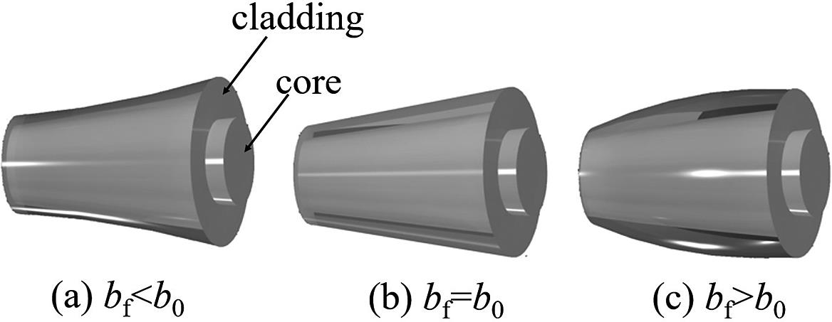
Fig. 2. Three major tapered categories: (a) concave tapered fiber, (b) linear tapered fiber, and (c) convex tapered fiber.
Fig. 3. Effects of different parabolic shape factors on the core radius profile (from the small end to the large end).
Fig. 4. Comparison of modal loss of straight T-SCF from the small end to the large end: (a) mode losses of LP01 and LP31e; (b) mode loss of LP11o.
Fig. 5. Comparison of modal loss of T-SCF with a bending radius of 32 cm: (a) mode losses of LP01 and LP31e; (b) mode loss of LP11o.
Fig. 6. (a) Modal loss and (b) effective mode area of LP01 for T-SCF under various bending azimuth angles, R = 32 cm, and z = 3.3 m.
Fig. 7. The amplifier model based on T-SCF under the small-to-large amplification scheme (the doped region colored red).
Fig. 8. Modal power evolution of (a) LP11 mode and (b) LP31e mode for concave, linear, and convex T-SCF based on the small-to-large amplification scheme.
Fig. 9. (a) Effective mode area of LP01 and (b) heat load density evolution along T-SCF.
Fig. 10. (a) Modal power evolution of four HOMs in linear T-SIF and (b) comparison of heat load density and effective mode area of LP01 between linear T-SCF and T-SIF.
Fig. 11. Power evolution of (a) LP11 mode and (b) LP31e mode in the T-SCF under a bending radius of 32 cm.
Fig. 12. Comparison of heat load density between straight T-SCF and bent T-SCF of R = 32 cm.
Fig. 13. The amplifier model based on T-SCF under the large-to-small amplification scheme (the doped region colored red).
Fig. 14. Modal power evolution of (a) LP11 mode and (b) LP31e mode for concave, linear, and convex T-SCF under the large-to-small amplification scheme.
Fig. 15. Comparison of heat load density between the two amplification schemes.
Fig. 16. Power of (a) LP11 and (b) LP31e of the T-SCF under a bending radius of 32 cm.
|
Table 1. The initial simulation parameters.


Set citation alerts for the article
Please enter your email address

© Copyright 2018-2021 | Chinese Laser Press. All Rights Reserved 沪ICP备15018463号-20