Hyperspectral Image Classification Based on Dilated Convolutional Attention Neural Network

Xiangdong Zhang; Tengjun Wang; Shaojun Zhu; Yun Yang

doi:10.3788/AOS202141.0310001

Journals >Acta Optica Sinica >Volume 41 >Issue 3 >Page 0310001 > Article

Acta Optica Sinica
Vol. 41, Issue 3, 0310001 (2021)

Hyperspectral Image Classification Based on Dilated Convolutional Attention Neural Network

Xiangdong Zhang^*, Tengjun Wang, Shaojun Zhu, and Yun Yang

Author Affiliations

School of Geology Engineering and Geomatics, Chang′an University, Xi′an, Shaanxi 710054, China

show less

DOI: 10.3788/AOS202141.0310001 Cite this Article Set citation alerts

Xiangdong Zhang, Tengjun Wang, Shaojun Zhu, Yun Yang. Hyperspectral Image Classification Based on Dilated Convolutional Attention Neural Network[J]. Acta Optica Sinica, 2021, 41(3): 0310001 Copy Citation Text

show less

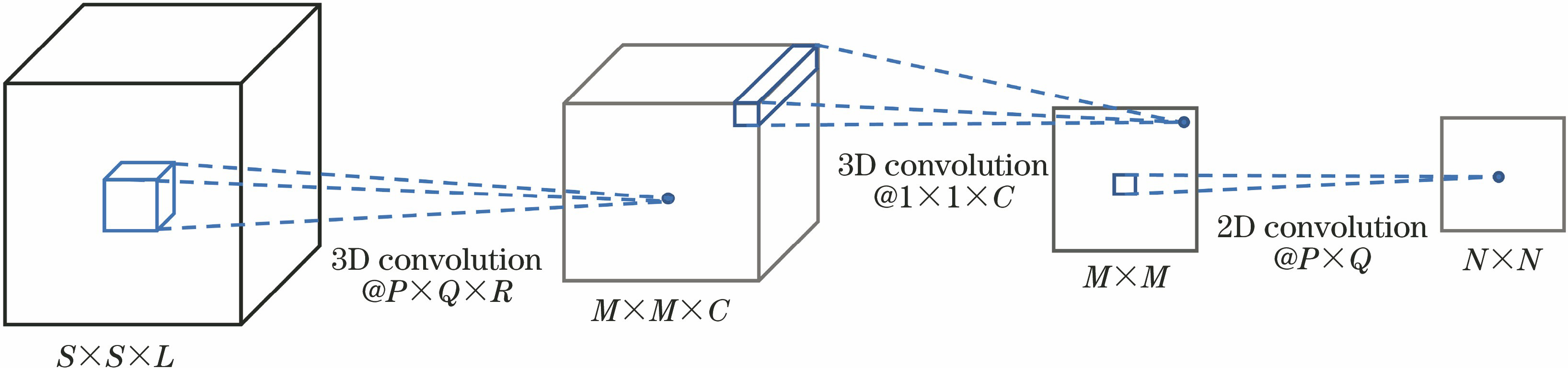
Fig. 1. Structure of tandem 3D-2D-CNN

Download full size

Schematic of standard convolution and dilated convolution. (a) 2D standard convolution; (b) 2D dilated convolution (r=2,2); (c) 3D standard convolution; (d) 3D dilated convolution (r=2,2,2)

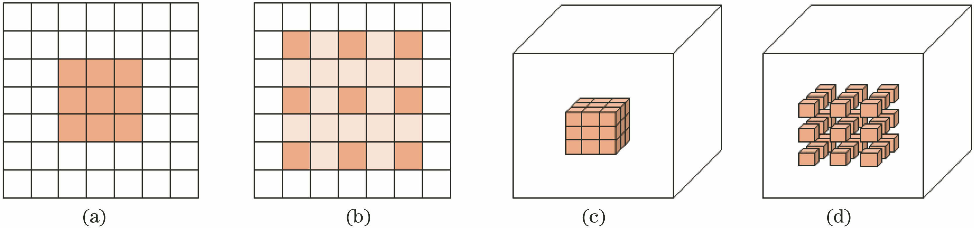
Fig. 2. Schematic of standard convolution and dilated convolution. (a) 2D standard convolution; (b) 2D dilated convolution (r=2,2); (c) 3D standard convolution; (d) 3D dilated convolution (r=2,2,2)

Download full size

Fig. 3. Multi-scale feature fusion structure. (a) Multi-scale spatial-spectral feature fusion module; (b) multi-scale spatial feature fusion module

Download full size

Fig. 4. Structure diagram of attention module. (a) Spatial-spectral attention module; (b) spatial attention module

Download full size

Fig. 5. Overall structure of proposed network

Download full size

Fig. 6. False color image and ground truth of data sets. (a) PU data set; (b) SA data set

Download full size

Fig. 7. Comparison of accuracy for different spatial sizes. (a) PU data set; (b) SA data set

Download full size

Fig. 8. Classification maps and partial enlarged maps with different algorithms on PU data set. (a) Ground truth image; (b) 2D-CNN-MLP; (c) 3D-CNN-CRF; (d) Hybrid-CNN; (e) Dilated-3D-CNN; (f) 3D-2D-ADCNN

Download full size

Fig. 9. Classification maps with different algorithms on SA data set. (a) Ground truth image; (b) 2D-CNN-MLP; (c) 3D-CNN-CRF; (d) Hybrid-CNN; (e) Dilated-3D-CNN; (f) 3D-2D-ADCNN

Download full size

Fig. 10. Overall accuracy with different numbers of training samples. (a) PU data set; (b) SA data set

Download full size

Kernel number	Pavia University			Salinas
Kernel number	OA /%	Training time /s	Test time /s	OA /%	Training time /s	Test time /s
16	97.78	118.03	29.71	96.48	243.42	66.38
20	96.87	130.56	34.19	97.28	324.71	76.93
24	97.17	149.93	38.34	96.26	373.57	88.24
28	96.25	185.74	43.35	95.88	383.83	98.84
32	97.05	165.58	46.76	96.12	416.47	107.36

Table 1. Comparison of overall accuracy, training time, and test time for different convolution kernel numbers

Architecture	Pavia University		Salinas
Architecture	Parameter	OA /%	Parameter	OA /%
3D-2D-CNN (baseline)	75596	98.11	139644	98.03
3D-2D-CNN+dilated convolution	56783	98.47	110402	98.42
3D-2D-CNN+attention	75643	98.51	139718	98.38
3D-2D-CNN+dilated convolution+attention	56857	98.73	110476	98.61

Table 2. Comparison of parameters and overall accuracy for different model architectures

Category name	2D-CNN-MLP	3D-CNN-CRF	Hybrid-CNN	Dilated-3D-CNN	3D-2D-ADCNN
Asphalt	87.33	86.78	90.89	84.86	96.82
Meadows	90.46	86.51	96.31	87.67	99.47
Gravels	84.91	85.76	94.45	87.73	99.35
Trees	93.00	96.27	92.39	97.71	97.77
Painted-Metal-Sheets	99.72	99.90	99.78	99.75	99.92
Bare-Soil	88.46	85.18	99.06	85.94	100.00
Bitumen	94.67	93.23	99.24	89.33	99.84
Self-Blocking-Bricks	85.04	86.74	87.81	83.76	98.91
Shadows	98.94	99.11	96.87	99.82	98.57
OA	89.76	87.92	94.89	89.48	98.75
AA	91.39	91.05	95.20	89.89	98.96
Kappa	96.54	84.22	93.26	86.04	98.60

Table 3. Comparison of classification accuracy for different algorithms on PU data setunit: %

Category name	2D-CNN-MLP	3D-CNN-CRF	Hybrid-CNN	Dilated-3D-CNN	3D-2D-ADCNN
Brocoli_green_weeds_1	99.98	99.39	99.99	99.97	100.00
Brocoli_green_weeds_2	99.48	98.92	99.96	99.70	100.00
Fallow	99.27	99.59	98.57	99.08	100.00
Fallow_rough_plow	99.30	99.16	99.47	99.47	99.61
Fallow_smooth	98.44	97.44	98.65	96.86	99.80
Stubble	99.76	99.94	99.79	99.76	100.00
Celery	99.61	99.60	99.84	99.60	100.00
Grapes_untrained	79.40	76.09	88.90	70.83	94.17
Soil_vinyard_develop	99.92	99.73	98.61	99.05	100.00
Corn_senesced_green_weeds	95.61	94.52	99.18	92.72	100.00
Lettuce_romaine_4wk	99.02	99.29	99.82	98.78	100.00
Lettuce_romaine_5wk	99.99	99.88	99.01	99.92	100.00
Lettuce_romaine_6wk	99.98	99.78	99.52	99.33	100.00
Lettuce_romaine_7wk	98.86	99.01	99.41	99.38	99.89
Vinyard_untrained	81.90	79.83	94.71	81.40	99.09
Vinyard_vertical_trellis	98.05	97.14	99.81	98.36	100.00
OA	92.57	91.38	96.48	90.25	98.61
AA	96.79	96.21	98.45	95.82	99.53
Kappa	91.73	90.40	96.09	89.17	98.45

Table 4. Comparison of classification accuracy for different algorithms on SA data setunit: %

Item	2D-CNN-MLP	3D-CNN-CRF	Hybrid-CNN	Dilated-3D-CNN	3D-2D-ADCNN
Parameter	33129	155017	4844793	413801	56857
Training time /s	8.91	103.30	63.75	671.89	122.22
Test time /s	2.17	13.04	7.85	72.36	51.93

Table 5. Comparison of parameters, training time, and test time for different algorithms on PU data set

Item	2D-CNN-MLP	3D-CNN-CRF	Hybrid-CNN	Dilated-3D-CNN	3D-2D-ADCNN
Parameter	33556	192144	4845696	498912	110476
Training time /s	16.94	276.08	97.08	2122.97	327.33
Test time /s	2.70	27.69	9.70	170.50	122.61

Table 6. Comparison of parameters, training time, and test time for different algorithms on SA data set

Xiangdong Zhang, Tengjun Wang, Shaojun Zhu, Yun Yang. Hyperspectral Image Classification Based on Dilated Convolutional Attention Neural Network[J]. Acta Optica Sinica, 2021, 41(3): 0310001

Download Citation

Set citation alerts for the article

Tools

Set citation alerts for the article

Save the article for my favorites

Paper Information