When we look at a three-dimensional (3-D) object in a conventional microscopy, we can only see a two-dimensional (2-D) projection at one time. Therefore, we need more information in order to extract the 3-D shape from the 2-D measurement. If we make a holographic measurement where we record both amplitude and phase, measuring at different z planes is equivalent to a single measurement followed by the digital propagation to multiple planes. Therefore, with coherent detection, a z-scan does not provide extra information compared to the single 2-D recording. Another dimension that can be exploited is the illumination angle θ. The measurements in the x, y, θ dimensions can be converted to the 3-D spatial domain by defining the physical relationship between the illuminating fields at the different angles and the corresponding measurements. However, most of the time, the 2-D measurements are incomplete due to the limited numerical apertures (NAs) of the optics, resulting in an inversion process that is highly ill-posed.

Optical diffraction tomography (ODT) is a 3-D imaging method that utilizes multiple 2-D measurements acquired by changing the angle of illumination. The contrast mechanism in ODT is endogenous index. It, therefore, does not require external labeling. ODT provides 3-D refractive index (RI) distributions¹ that contain morphological and biochemical information, which have been widely used to study various biological samples, which are summarized in recent review papers.^2–5 Under the assumption of weak scattering, multiple 2-D measurements in (x,y,θ) can be directly inverted to yield the 3-D RI information in (x,y,z) using the Wolf transform,⁶ which is the transformation that maps the spatial frequencies of the 2-D spectrum of the projections to the spatial frequencies of the 3-D spectrum of the object. However, direct inversion reconstruction methods based on the Wolf transform suffer from the missing cone problem—a consequence of the missing spatial frequencies that are not accessible due to the limited NAs of the optics.⁷

The missing cone problem has been intensively investigated due to its importance.^7,8 Previous approaches are model-based iterative reconstruction (MBIR) schemes, which exploit regularizations based on our prior knowledge, such as non-negativity or sparsity constraints. In other words, MBIR schemes find a solution that is not only consistent with the measurements but also sparse in the regularization domain. The choice of regularization is critical. However, it requires extensive understanding of the characteristics of the forward models, including the degree of ill-posedness intertwined with the characteristics of the samples. This makes the problem challenging.

Recently, deep neural networks (DNNs) have been successful in various optical applications, such as enhancement of the transverse resolution,⁹ phase retrieval from intensity measurements,^10,11 digital staining,^12,13 classification/segmentation based on holographic/tomographic measurements,^14–16 and others.^10,17,18 There are some previous demonstrations of the benefits of applying DNNs to the reconstruction of RI values in ODT.^19–21 As far as we know, nobody has succeeded before in using DNNs to reconstruct arbitrary 3-D RI distributions from limited angle measurements taking diffraction and multiple scattering into account.

In this paper, we describe a method based on DNNs to solve the long-standing missing cone problem and demonstrate it using red blood cell (RBC) samples. Despite the potential capacity of DNNs, the lack of the ground truth prevents us from applying DNNs on the ODT reconstruction, unlike other DNN optical imaging applications, such as digital staining or phase retrieval where we can access the target images. Our approach relies on the formation of digital phantoms followed by accurate digital models, which provide the 2-D measurements. The digital 2-D projections are used to form a rough 3-D image of the object using the Wolf transform under the Rytov approximation.⁶ By training a DNN with the pairs of images from the Wolf transform and the corresponding digital phantoms, we can learn the distortions introduced due to the incomplete measurements in a data-driven way.

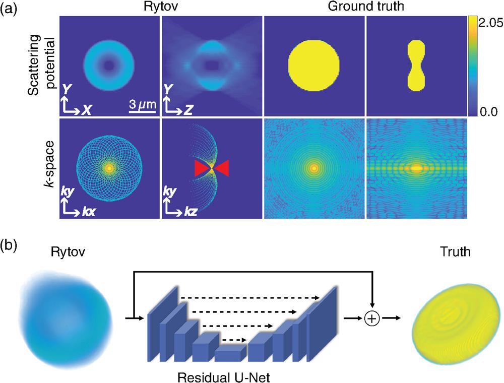
We demonstrate the method by using RBC samples that are highly affected by the missing cone problem. The shape of RBCs is flat and biconcave showing narrow dimple regions at the center, which requires high-frequency components along the optical axis to fully resolve the structures.^22,23 In Fig. 1(a), we observe that cross sections of the Rytov reconstruction are underestimated and elongated along the z axis when compared with the corresponding sections of the ground truth. The k-space representation of the Rytov reconstruction can be considered as the low-pass filtered version of the k-space of the ground truth under the weak scattering assumption. Looking at the k-space of the ground truth, the frequency components are more broadly distributed in the kz axis compared to ones in the ky axis since the sample is broad in the y axis but has the narrow biconcave shape in the z axis. While high-frequency components are required to fully resolve the thin structure, most of them are lost because they are inaccessible due to the limited NAs as indicated by the red triangles. This results in the high distortions in the final Rytov reconstruction. In general, Rytov reconstructions of RBCs show holes in the middle making it hard to retrieve meaningful information, such as cell volume, surface, and RI values.

A DNN can be trained to recover those missing high frequencies, which are especially important for forming tomograms of RBCs. The network reconstructs the original RBC with the Rytov reconstruction as the initial condition in the training of the DNN, as shown in Fig. 1(b). We refer to the network as TomoNet throughout this paper. The input to the network is the Rytov reconstruction of an RBC and the output is the enhanced image of the same RBC. The input is also relayed directly to the output of the network where it is summed with the correction calculated by the DNN. Therefore, the network learns to extract the difference between the input and the output. In other words, given the low-pass filtered input, the network synthesizes the missing high-pass filtered information using data-driven features from a large number of examples. By combining the low-pass filtered input with the high-pass synthesized output from the network, we can achieve the full resolutions in the transverse and axial planes.

For training, we digitally generated many RBCs that are different in shape and RI value using the RBC model, as shown in Fig. 2(a).²⁴ For detailed information of the generation of different RBCs, we refer interested readers to Appendix A. Then, each RBC served as a sample for DDA simulations to generate accurate synthetic measurements, as shown in Fig. 2(b).^25,26 A total of 40 uniformly spaced measurements were acquired by scanning on a circular pattern while maintaining a fixed illumination angle of 36 deg with respect to the z axis. The RBC phantoms generated using the model ^[Fig. 2(a)] originally lie in the xy plane. We implemented the various orientations of RBCs that can occur by randomly rotating each sample in the yz and xy planes. The DDA method was then used to calculate the 2-D projections of each 3-D phantom for each of the 40 illumination angles ^[Fig. 2(c)]. These calculations were used to form 3-D reconstructions using the Rytov method, which served as the input to the network.⁶ Each Rytov reconstruction was paired with the corresponding synthetic RBC that was used to generate the calculations. Figure 2(c) shows two example pairs, one without rotation and the other with rotation.

For each RBC pair, we want to augment the dataset by shifting each example in all the axes. To do so, it is important to consider the shift properties of the Rytov reconstruction along each axis. We start from the integral solution to the Helmholtz equation: where F(r)=k2/4π[n(r)2/n02−1] is the scattering potential of a sample whose RI distributions are n(r) when immersed in a medium whose RI is n0, given a wavenumber for the wavelength λ in vacuum, k=2πn0/λ. Here G(r−r′)=e1ik|r−r′|/|r−r′| is the Green’s function of the 3-D Helmholtz equation. The Ui(r) and U(r) are the incident and total electric fields, respectively, and the Us(r) is the scattered electric field, Us(r)=U(r)−Ui(r). The term Us, on the left-hand side, can be measured at the image plane, as shown in Fig. 2(d). It is intuitive to see that moving the sample in the xy plane results in the same shift in the plane of the measurement of the scattered field. When the sample is translated in z, however, the measured scattered field will be the propagated version of the original unshifted measurement. Assuming that the sample is weakly scattering, the Rytov approximation uses the phase of the field itself, and Eq. (1) can be rewritten as follows: The left term of Eq. (1), U(r)−Ui(r)=[elogU(r)/Ui(r)−1]Ui(r), is replaced with the first Taylor expansion of it, Ui(r)logU(r)/Ui(r). It, therefore, loses the propagation property of the scattered field. We refer this term as Us−Rytov. In other words, we must recalculate Us−Rytovz−shift when an object is shifted in the z axis and the result of this calculation is different than distally propagating the field Us−Rytov.

Taking these properties into consideration, we augmented the set of training examples by generalizing shifted versions of the original pairs. For the shift in the xy plane, we added an xy-shifted version of each pair in addition to the original pair (without any shift). The shift was randomly selected during training. For the shift in the z axis, after generating the 40 projections for an RBC centered at z=0, we digitally propagated the simulated measurements, U and Ui, to four different z planes (−2Δz, −Δz, +Δz, and +2Δz) and calculated the corresponding Us−Rytov values at each plane. This was followed by their Rytov reconstructions to obtain examples of RBCs shifted along the z axis. In this work, Δz was set to 122 nm, which corresponds to one pixel of reconstruction grid. Rytov reconstructions were paired with the shifted RBCs in the z axis.

We trained a U-Net-type DNN in the regression manner using the following weighted l2-norm as the cost function:^27,28Error(xrecon,xtrue)=‖xrecon−xtrue‖22‖xtrue‖22,(3)where xrecon is the output from the network given xRytov, and xtrue is calculated from the ground truth RI contrast. Here, x represents the RI contrast multiplied by a scalar value, which is calculated as c(n−n0), where n represents sample RI distributions and n0 is the RI of medium. The scalar c was introduced for normalization of values; c can be either 40 for xRytov or 20 for xtrue. Negative components of input and output of the network were discarded. We implemented the network using PyTorch (1.2.0) and compute unified device architecture toolkit (10.0) on a desktop computer (Intel Core i7-6700 CPU, 3.4 GHz, 32 GB RAM) with a graphic processing unit (GPU, GeForce GTX 1070). The network was trained using the Adam optimizer with the learning rate of 1×10−4, and it decayed half after every 10 epochs.²⁹ The mini-batch size was 8 and the total number of epoch was 50.

Figure 3 describes the network structure. It is very similar to the U-Net proposed in Refs. 27 and 28, except for slight modifications.^30,31 The input is skip-connected and summed to the output of the network. Therefore, the network learns the residual difference between the Rytov reconstruction and the ground truth.²⁸ All biases in the convolutional layers were set to zero and fixed. Zeros were padded for convolution layers of which kernel sizes are bigger than 1 so that the dimensions stay equal before and after the convolutions. The negative slope of leaky rectified linear unit (RELU) was set to 0.01. For the normalization layer, affine transform was turned off. For the transpose convolutional layers, the kernel size was set to 6×6×6 with the zero padding of 2×2×2 and the stride of 2×2×2.

The optical setup is described in Fig. 4.³² It includes a diode pumped solid state 532 nm laser. The laser beam was first spatially filtered using a pinhole spatial filter. A beamsplitter was used to split the input beam into a sample beam and a reference beam. The sample beam was directed onto the sample at different angles of incidence using a reflective liquid crystal on silicon spatial light modulator (SLM) (Holoeye) with a pixel size and resolution of 1080×1920pixels. Different illumination angles were obtained by projecting blazed gratings on the SLM. In the experiment presented here, a blazed grating with a period of 25 pixels was rotated a full 360 deg. Two 4F systems between the SLM and the sample permitted filtering of higher orders reflected from the SLM (due to limited fill factor and efficiency of the device) as well as magnification of the SLM projections onto the sample. Using a 100× oil immersion objective lens with NA 1.4 (Olympus), the incident angle on the sample corresponding to the grating was 36 deg. The magnification of the illumination side was defined by the 4F systems we used before the sample. A third 4F system after the sample includes a 100× oil immersion objective lens with NA 1.45 (Olympus). The sample and reference beams were collected on a second beamsplitter and projected onto a scientific CMOS (sCMOS) camera (Neo, Andor) with a pixel size and resolution of 2150×2650pixels.

Blood sampling was performed by terminal intracardiac puncture on wild-type Balb/cByJ adult mice, in agreement with the Swiss legislation on animal experimentation (authorization number VD3290). RBCs were then isolated from blood plasma by centrifuging using Eppendorf-Centrifuge 5418 at 400 rpm for 3 min. RBCs were then fixed using glutaraldehyde with concentration of 0.25% in phosphate-buffered saline (PBS) followed by centrifuging for 1 min and washing three times with PBS to remove any fixation reagents traces. To ensure strong adhesion between the RBC and the coverslip, coverslip was coated with 0.1% poly L-lysine diluted in PBS with molecular weight ranging between 1000 and 5000gm/mol.

Results obtained with the TomoNet are displayed in Fig. 5 for two different RBCs. Here, we only present centered RBCs without shifts in the xy plane. The first row shows RI reconstructions of Rytov, TomoNet, and the ground truth. The second row displays the difference map from the ground truth (reconstruction – the ground truth). In other words, blue regions in the difference map display underestimated parts and yellow regions show elongated regions. As expected, the Rytov reconstructions underestimate the RI values and elongate the RI distributions along the optical axis. Especially, the central dimple region of the RBC is significantly deteriorated. This is because the dimple region is thin and requires high frequencies for its reconstruction. By contrast, TomoNet shows excellent reconstruction results since it estimates accurately the values of these high frequencies from the data in the training set. In other words, the TomoNet implements super-resolution for 3-D samples revealing spatial details beyond the classical resolution limit. We quantitatively assessed the accuracy of the TomoNet over the Rytov reconstruction by calculating the following metric: error(Δnrecon,Δntrue)=‖Δnrecon−Δntrue‖22‖Δntrue‖22,(4)where Δnrecon is the reconstructed RI contrast and Δntrue is the ground truth RI contrast. Here, Δn represents the RI contrast, which is defined as (n−n0), where n represents the sample RI distributions and n0 is the RI of medium. We discarded the negative values when calculating the error metric. The mean error values over all test RBCs are 0.5929 for the Rytov method and 0.0084 for the TomoNet, which confirms the improved performance of the network. The trained network accurately reconstructs RBCs and it does so in less than 10 ms on a GPU (GeForce GTX 1070).

We applied the network trained with digital phantoms to the Rytov reconstruction of a mouse RBC formed from experimental measurements. In the experiment, the samples were circularly scanned at the illumination angle of 36 deg in 9-deg steps resulting in 40 measurements, matching the parameters we used to generate the digital training data. As shown in Fig. 6, the Rytov reconstructions using the measurements show severe distortions, especially at the dimple region as we also observed in the synthetic data. With the Rytov reconstruction as its input, the TomoNet reconstructs RI tomograms without those artifacts resulting in the biconcave morphology. We verified the great improvement in the quality of the reconstructions visible in Fig. 6, by using a quantitative method³³ to evaluate the reconstruction accuracy of 3-D objects when the ground truth is not accessible. This was possible by generating semisynthetic measurements.

As described in Fig. 7(a), following the reconstruction of the RI distributions from the experimental measurements, we generated semisynthetic 2-D projections using an accurate forward model such as the DDA at each illumination angle. By comparing the digital projections with the corresponding 2-D experimental measurements, the difference between them reflects how close the 3-D reconstruction is to the ground truth. It is noteworthy that we did not use the forward model involved in the reconstruction to generate the digital projections to be fair.

Figure 7(a) shows two examples of phase maps from digital projections. For each digital projection, we calculated the projection error map, the difference in phase information between experimental and simulated measurements, along with the mean projection error map over all angles. Figure 7(b) displays two randomly selected projection error maps as well as the mean projection error maps for the Rytov and the TomoNet. In the case of Rytov, we can clearly see the mismatch between experimental and digital projections in the mean projection error map. By contrast, the mean projection error map of TomoNet shows excellent consistency. We further quantitatively confirmed the improvement in performance of TomoNet over Rytov by calculating the metric, ∑l=1L‖ρexpl−ρsynl‖2/N, where L is the total number of angles, N is the total number of pixels, and ρexp and ρsyn are the phase maps from experimental and semisynthetic measurements, respectively. As shown in Fig. 7(b), the average of the metric shows twofold improvement of TomoNet over the Rytov method.

We presented a DNN approach for reconstructing tomograms of RBCs with greatly improved image quality and super-resolution capability, especially enhancing the axial resolution. We digitally generated various RBCs and used them to generate synthetic measurements using the DDA to overcome the lack of the ground truth. The network trained on the synthetic data accurately reconstructs RI distributions of RBCs resolving the problems caused by the missing cone problem. We applied the trained network on experimental data to utilize extracted features from the synthetic datasets. Despite the lack of the ground truth for the experimental result, we further validated the result of the network using semisynthetic measurements, and it confirmed the great improvement.

In this work, we focused on one specific cell type, RBCs, since it is relatively easy to model them. More importantly, RBCs are highly distorted by the missing cone problem, which prevents us from retrieving meaningful information for various applications. However, we believe that the proposed scheme can be further extended to other types of sample by carefully designing phantoms to statistically capture information in the generated dataset.

The shape of the surface of an RBC can be modeled by the following equation: where ρ is the radius in cylindrical coordinates (ρ2=x2+y2) and S, P, Q, and R are the parameters derived from d, h, b, and c shown in Fig. 2(a).²⁴ To generate various RBCs, the d, h, and b values in microns were randomly selected from normal Gaussian distributions whose mean values were 7.65, 2.84, and 1.44 and standard deviations were 0.67, 0.46, and 0.47. c/d and the normalized RI values, (n−n0)/n0, were sampled from uniform distributions whose ranges were (0.56, 0.76) for c and (1.0355, 1.596) for the normalized RI.²⁴ To avoid nonrealistic shapes, several criteria were applied to limit the parameter values in the following ranges: h<0.95×d/2 and b≤h. In addition, we limited the derived geometrical parameters such as cell volume (Vμm3), surface (Sμm2), and sphericity index (SI), 6πV/S3/2, to fall within the normal ranges: 66<V<130, 98<S<162, and 0.494<SI<0.914.²⁴ The cell surface was calculated using the equation, πd[d/2+2h×(sinh−1e)/e], where e=29d2−4h2/5h.³⁴ Finally, RBC shapes were downsampled with a factor, 7.65/5.8, since the mean diameter of mouse RBCs is 5.8μm, compared to the 7.65μm for humans.³⁵ A total of 100 different RBCs were generated and each of them was randomly rotated in the yz plane (uniform distribution: [0, π/6]) and the xy plane (uniform distribution: [0, 2π]) resulting in 200 different RBCs (100 without rotation and 100 with rotation).

To generate synthetic measurements using the DDA, each RBC was illuminated at the incident angle of 36 deg for 40 angles, which were uniformly distributed on a circle. The illumination wavelength λ was 396 nm and the size of each dipole was set to λ/12=33nm. The background medium in the simulation was air and the sample RI was set to the normalized RI. For 2-D measurements, the size of the grid was 256×256 with a pixel size of 99 nm. After that, the measurements were downsampled by cropping in k-space resulting in a pixel size of 122 nm. The original phantom defined using dipoles interpolated to a sampling grid that matched the pixel size of the measurements.

Measurements for 200 randomly generated RBCs were digitally refocused to five different planes resulting in 1000 pairs. Totally 800, 100, and 100 pairs were used for training, validation, and test, respectively. For the training and validation, we doubled the datasets by adding the randomly shifted sets on top of the original sets, resulting in 1600 and 200 pairs. The random shift varied at every iteration. For the rotated RBCs, after generating the measurements, we reversely rotated the Rytov reconstructions and the paired ground truth RBCs in the xy plane, resulting in rotations only in the yz plane to simplify the training. For the experimental data, since we do not know the rotation angle in the xy plane, we applied ellipsoidal fitting on a binary mask generated by applying Otsu thresholding³⁶ on the maximum projection map of Rytov. By analyzing the short and long axes, we extracted the orientation of the RBC. Since the Rytov reconstruction is shift-invariant in the xy plane, we simply interpolated in the xy plane for rotation.

The semisynthetic measurements were calculated using reconstruction results acquired from Rytov and TomoNet as samples for the DDA simulations. The pixel size of these reconstructions was 122 nm. Since the size of dipole was set to λ/6n0=67nm, where λ=532nm and n0=1.334, the reconstructions were interpolated to a grid, one pixel of which was the size of a dipole. Then, we discretized the RI values as round(n/n0×1000)/1000, and the negative values were discarded.

References

[1] M. Born, E. Wolf. Principles of Optics: Electromagnetic Theory of Propagation, Interference and Diffraction of Light(1999).