Adaptive window iteration algorithm for enhancing 3D shape recovery from image focus

Long Li; Zhiyan Pan; Haoyang Cui; Jiaorong Liu; Shenchen Yang; Lilan Liu; Yingzhong Tian; Wenbin Wang

doi:10.3788/COL201917.061001

Abstract

Depth from focus (DFF) is a technique for estimating the depth and three-dimensional (3D) shape of an object from a multi-focus image sequence. At present, focus evaluation algorithms based on DFF technology will always cause inaccuracies in deep map recovery from image focus. There are two main reasons behind this issue. The first is that the window size of the focus evaluation operator has been fixed. Therefore, for some pixels, enough neighbor information cannot be covered in a fixed window and is easily disturbed by noise, which results in distortion of the model. For other pixels, the fixed window is too large, which increases the computational burden. The second is the level of difficulty to get the full focus pixels, even though the focus evaluation calculation in the actual calculation process has been completed. In order to overcome these problems, an adaptive window iteration algorithm is proposed to enhance image focus for accurate depth estimation. This algorithm will automatically adjust the window size based on gray differences in a window that aims to solve the fixed window problem. Besides that, it will also iterate evaluation values to enhance the focus evaluation of each pixel. Comparative analysis of the evaluation indicators and model quality has shown the effectiveness of the proposed adaptive window iteration algorithm.

With the development of high-precision measurement technology, it is an important research direction to make non-contact and high-precision measurement of the surface morphology of microscopic objects by using high-resolution microscopic images. Three-dimensional (3D) reconstruction distortion is the common problem in the field of image measurement, especially when multi-focus microscopic image measurement is more prominent, and distortion of the 3D reconstruction model will seriously affect the measurement results. Depth from focus (DFF) deals with the recovery of 3D shapes from multi-focus image sequences^[1,2]. DFF requires searching the best focus setting that gives the best focus at each point^[3,4]. Thus, each pixel point of an object is required to be well focused in multi-focus image sequences. According to the current research status, Mahmood et al. proposed a non-linear filtering method to enhance the focus volume for accurate depth estimation^[5]. Lee et al. proposed an adaptive window algorithm to enhance the focus measure, where the algorithm adjusts the window size based on median absolute deviation^[6]. Mahmood et al. used the most basic operator for calculation, but optimized the genetic algorithm for fitting the focus curve to a height curve^[7]. Leach explained the principle of Alicona equipment and provided a complete solution for the selection of lighting methods, the selection of the interpolation fitting algorithm of the focus evaluation function, and the way of dealing with the noise in the model^[8]. Aydin and Akgul suggested an adoptive weighted window that adjusts the weights using the information from an all-in-focus image. Thelen discussed the importance of the window size and suggested an algorithm for the second stage that selects the effective window size from several neighborhood sizes based on confidence criterion^[9]. All methods of focus evaluation measurement mentioned above only use a fixed window without considering the impact of iterative evaluation for depth estimation. In this Letter, we discuss the issue of window selection and enhanced focus evaluation to recover 3D shapes from the image focus accurately.

There are two main causes of distortion in 3D reconstruction. The first is the absence of much consideration in the evaluation of focus pixels during the evaluation process at the pixel point, and the second is the window size on the focus evaluation operator being fixed, e.g., $3 \times 3$ , $5 \times 5$ . Thus, for some pixels, enough neighbor information cannot be covered in the fixed window and easily interfered with by noise, which results in distortion of the model. For other pixels, the fixed window is too large, which increases the computational burden.

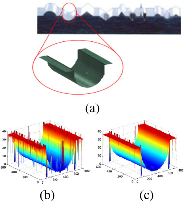
For example, we use the modified Laplacian ( ${FM}_{SML}$ ) to reconstruct the profile of semi-cylindrical model in the Alicona standard block. Two causes of distortion in the reconstruction of the specific form of the model are shown in Fig. 1.

Sign up for Chinese Optics Letters TOC. Get the latest issue of Chinese Optics Letters delivered right to you！Sign up now

Figure 1.Depth maps of semi-cylindrical model. (a) Alicona semi-cylinder standard model, (b) semi-cylinder using window size $3 \times 3$ , (c) semi-cylinder using window size $5 \times 5$ .

Figure 1(b) shows the obvious distortion of the semi-cylinder reconstruction using the window $3 \times 3$ , while the distortion of the reconstruction model is partly improved using the window $5 \times 5$ . Although the increase in the window will improve the reconstruction distortion to a certain extent, it will greatly increase computational burden. From the results of the experiment in Figs. 1(b) and 1(c), the full focus pixel point cannot be accurately obtained by one time focus evaluation.

Therefore, the adaptive window iteration algorithm is proposed to enhance the image focus with the aim of producing accurate depth estimation.

Human consideration in determining the clarity of the image is only limited to information captured by the eye. However, the computer uses the focus evaluation algorithm to determine the degree of focus of the image^[10,11]. Because the precision mobile platform moves in the $Z$ direction and the measured area of the object passes through the depth of field of the microscope objective, the measured area of the object will inevitably undergo “out of focus almost in focus–in focus–almost in focus–out of focus”^[12,13].

A focus measure is defined as the quantity for locally evaluating the sharpness of a pixel. It takes the small local neighborhood and computes the sharpness of a chosen center pixel. Since each object point has different surface characteristics and geometry, the values of the focus measure of the same object point from different optical settings are compared. Some popular algorithms have been applied to measure contrast, and one of them is the gray-level variance (GLV). It comes from the principle that high variance is intuitively associated with sharp image structure, while low variance is associated with blurring, which reduces the amount of gray-level fluctuation^[14,15]. Therefore, GLV focus measure can be obtained by taking the variance of the gray-level values of pixels within a local window as ${FM}_{GLV} (x, y) = \sum_{(i, j) \in W_{n \times n}} {[I (x, y) - μ]}^{2},$ (1)where $W_{n \times n}$ is the local window with the size of $n \times n$ centered at $(x, y)$ , $I (x, y)$ is the value of the pixel $(x, y)$ , and $μ$ is the mean value of pixels in $W_{n \times n}$ .

Another type of method is based on derivatives. The Tenegrad focus measure (TEN)^[16,17] is a gradient magnitude maximization method that measures the sum of the squared responses of the horizontal and vertical Sobel masks, shown in the following: ${FM}_{TEN} (x, y) = \sum_{(i, j) \in W_{n \times n}} [G_{x} {(x, y)}^{2} + G_{y} {(x, y)}^{2}],$ (2)where $G_{x}$ and $G_{y}$ are the $X$ and $Y$ image gradients, respectively, computed by convolving the given image $I$ with the Sobel operators.

The Laplace operator, a second-order differential operator in the n-dimensional Euclidean space, is defined as the divergence ( $\nabla$ ) of the gradient $(\nabla f)$ . Thus, if $f$ is a twice-differentiable real valued function, then the Laplacian of $f$ is defined by $Δ f = \nabla^{2} f = \nabla \cdot \nabla f$ . The latter notations derive from formally writing $\nabla = (\frac{\partial}{\partial x_{1}}, \dots, \frac{\partial}{\partial x_{n}})$ , and the Laplace operator in two dimensions is given by $\nabla f = \frac{\partial^{2} f}{\partial x^{2}} + \frac{\partial^{2} f}{\partial y^{2}}$ . The Laplace operator, being a point and symmetric operator, is suitable for accurate shape recovery. Unlike the previous first-derivative-based gradient function, the Laplace operator uses the second derivative as the basis. The reason is that the second derivative can be further amplified compared to the first derivative to change the value of the function and extract the high-frequency components more accurately. In the original form of the Laplace operator, the second-order partial derivative of the $x$ direction and the $y$ direction may be opposite to each other, offset one another, and produce deviations in the focus of the image

In order to solve the problem of zero Laplacian value and improve its robustness for weak-textured images, this operator is reformulated by Nayar and Nakagawa^[16,17] to get a new equation, namely, the sum of the modified Laplacian (SML) as ${FM}_{SML} (x, y) = \sum_{(i, j) \in W_{n \times n}} [{(\frac{\partial^{2} g (x, y)}{\partial x^{2}})}^{2} + {(\frac{\partial^{2} g (x, y)}{\partial y^{2}})}^{2}] .$ (3)

To further simplify it, the discrete approximation to Eq. (3) is launched, and a variable spacing step to accommodate for possible variations in the texture element sizes is also added^[18–20]. Therefore, the equation is shown as $ML (x, y) = | 2 I (x, y) - I (x - step, y) - I (x + step, y) | + | 2 I (x, y) - I (x, y - step) - I (x, y + step) |,$ (4) ${FM}_{SML} (x, y) = \sum_{(i, j) \in W_{n \times n}} ML (x, y) for ML (x, y) \geq T,$ (5)where $T$ is a threshold. The higher quality the input image sequence possesses, the shorter step is the better one to use.

In order to enhance the ability of focus evaluation to obtain an accurate 3D model, the adaptive window iteration algorithm is proposed in this Letter. The algorithm is divided into two parts: in the first part, an adaptive window algorithm is used to calculate the size of each pixel corresponding to the window; in the second part, the iteration of the focus evaluation value is performed within each pixel window.

(1) Adaptive window algorithm

The adaptive window algorithm can automatically adjust the size of the window according to the neighboring chromatic aberrations of a pixel. Because of the neighboring chromatic aberrations, calculation of color images will increase computational burden. Therefore, this algorithm will convert color images to gray images and then calculate the neighboring chromatic aberrations of a pixel. In Fig. 2(a), the window size for both Pixels 1 and 2 is the same, as shown in Fig. 2(b), and calculating the window size of Pixel 2 with less neighboring chromatic aberration than Pixel 1 is appropriately expanded to improve the accuracy in the 3D model recovery until an upper limit of the window size is met. Similarly, in order to reduce computational volume, the window size of Pixel 1 is decreased before the chromatic aberration meets a lower limit.

Figure 2.Principle of algorithm for adaptive window size.

Specific steps to achieve the adaptive algorithm are as follows.Step 1: Set the initial window size to $P (Eg 9 \times 9)$ . Set the maximum value of window size to $P_{\max} (Eg 17 \times 17)$ and the minimum value of window size to $P_{\min} (Eg 3 \times 3)$ .Step 2: Use the initial window for image fusion based on time domain.Step 3: Convert time-domain fused color images to gray images and then calculate the overall average deviation ( ${\bar{A}}_{total}$ ) of each pixel and average deviation [ $\bar{A} (x, y)$ ]of each pixel in the initial window of the time-domain fused image. Image size is $N \times M$ , initial window size is $n \times n$ : ${\bar{A}}_{total} = \frac{\sum_{(x, y) \in W_{N \times M}} \bar{A} (x, y)}{N \times M} = \frac{\sum_{(x, y) \in W_{N \times M}} [f (x, y) - \frac{\sum_{(i, j) \in W_{n \times n}} f (x_{i}, y_{j})}{n^{2}}]}{N \times M} .$ (6)Step 4: Updated window. ① if ( $\bar{A} (x, y) > {\bar{A}}_{total}$ ) ⊳Compare $\bar{A} (x, y)$ with ${\bar{A}}_{total}$ ② if ( $P > P_{\min}$ ) ⊳Compare $P$ with $P_{\min}$ ③ $W_{n \times n} (x, y) = P - 1$ else $W_{n \times n} (x, y) = P$ ⊳Update window size to $W_{n \times n} (x, y)$ ④ else if ( $\bar{A} (x, y) < {\bar{A}}_{total}$ ) ⊳Compare $\bar{A} (x, y)$ with ${\bar{A}}_{total}$ ⑤ if ( $P < P_{\max}$ ) ⊳Compare $P$ with $P_{\max}$ ⑥ $W_{n \times n} (x, y) = P + 1$ else $W_{n \times n} (x, y) = P$ ⊳Update window size to $W_{n \times n} (x, y)$ Step 5: Repeat the above steps to determine the window size for each pixel.

(2) Iteration algorithm of focus evaluation value

In Figs. 3(a) and 3(b), the image focuses on one area instead of one point due to the depth of field of the microscope. Therefore, the focus evaluation value of each pixel located in the focus area is the largest in the image sequence. A new value of the focus evaluation will be obtained by adding the focus evaluation value of the center of the pixel with the focus evaluation value of the other pixels in the window. By repeating this iteration process, the highest degree of focus pixels in the image sequence can be obtained. Thus, the new focus evaluation values ${FM}^{*}$ after iteration will be gained: ${FM}^{*} (x, y) = \sum_{(i, j) \in W_{n \times n} (x, y)}^{N} [FM (x, y, k)], 1 \leq k \leq K,$ (7)where $N$ is the iteration number, $W_{n \times n} (x, y)$ is the window size of the pixel $(x, y)$ , and $K$ is the total number of image frames.

Figure 3.Image focus evaluation process. (a) Image sequence acquisition, (b) regional focus, (c) fitting focus evaluation curve.

For each image frame $k$ from the total of $K$ image frames, the focus measure $FM (x, y, k)$ is computed at each pixel $(x, y, k)$ in the acquired image sequences by applying a focus measure on the adaptive window centered at $(x, y, k)$ . Then, for the point $(x, y)$ , the $depth (x, y)$ is computed by taking the frame number that produces the maximum focus measure from $FM (x, y, k)$ : $depth (x, y) = \underset{k}{argmax} [FM (x, y, k)], 1 \leq k \leq K .$ (8)

Because image sequence $I$ is discrete, the focus evaluation curve of pixel $(x, y)$ in the sequence of images consists of discrete points. Therefore, this algorithm uses the polynomial curve fitting method to get a more accurate peak position. The focusing evaluation curve is shown in Fig. 3(c)^[8], so we use a polynomial fit to the point near the maximum, as shown in Eq. (9): $p (z) = a Z^{2} + b Z + c .$ (9)

The exact peak position can be calculated by using the coefficients $a$ and $b$ , $Z = - \frac{b}{2 a}$ .

We compare the reconstruction model of the $N$ th iteration with the reconstruction model of the ( $N - 1$ )th iteration. Note that at steady state, the high difference (HD) between $Z^{(N)} (x, y)$ and $Z^{(N - 1)} (x, y)$ becomes very small. So, the HD termination criterion can be written as $HD = {{[Z^{(N)} (x, y) - Z^{(N - 1)} (x, y)]}^{2}}^{1 / 2} \leq δ .$ (10)

During experimentation, for objects with bevel angles closer to 90°, we found the value $δ = 2$ . In other situations, value $δ \leq 1$ .

Figure 4 is the block diagram of an adaptive window iteration algorithm.

Figure 4.Block diagram of the adaptive window iteration algorithm. (a) Calculate the window size for each pixel, (b) focus evaluation iteration.

The experimental platform of this Letter is the HP Z620 workstation, the operating system is Windows 10, and the software is MATLAB 2011b. The reconstruction object of this experiment is the profile of the slope, triangle, and semi-cylinder in the Alicona morphology standard block, shown in Fig. 5. Table 1 shows the experimental image acquisition parameters. In order to compare the performance of different focus measures quantitatively, the root mean square error (RMSE), peak signal-to-noise ratio (PSNR), and correlation coefficient (CC)^[6,21] are used. If $f (x, y)$ is the original image, and $g (x, y)$ is the processed image, then the RMSE, PSNR, and CC are calculated as follows: $RMSE = \sqrt{\frac{1}{X Y} \sum_{x = 0}^{X - 1} \sum_{y = 0}^{Y - 1} {| f (x, y) - g (x, y) |}^{2}},$ (11) $PSNR = 10 \times \log_{10} \frac{X Y [\max f (x, y) - \min f (x, y)]}{\sum_{x = 1}^{X} \sum_{y = 1}^{Y} {[g (x, y) - f (x, y)]}^{2}},$ (12) $CC = \frac{\sum_{x = 1}^{X} \sum_{y = 1}^{Y} [f (x, y) - \bar{f}] [g (x, y) - \bar{g}]}{\sqrt{{\sum_{x = 1}^{X} \sum_{y = 1}^{Y} {[f (x, y) - \bar{f}]}^{2}} {\sum_{x = 1}^{X} \sum_{y = 1}^{Y} {[g (x, y) - \bar{g}]}^{2}}}} .$ (13)

	Acquisition Parameters
Object	Magnification	Lighting Method	Adjacent Image Distance (μm)	Image Size	Image Number
Slope	5×	Dark field	10	672×378	37
Triangle	5×	Dark field	10	812×616	46
Semi-cylinder	5×	Dark field	10	791×600	40

Table 1. Optical Conditions and Acquisition Environment

View all Tables

Figure 5.Reconstruct the object. (a) Triangle, (b) slope, (c) semi-cylinder.

Figure 6 shows depth maps obtained by three groups of focus measure operators ( ${FM}_{GLV}$ , ${FM}_{GLV}^{*}$ ), ( ${FM}_{TEN}$ , ${FM}_{TEN}^{*}$ ), and ( ${FM}_{SML}$ , ${FM}_{SML}^{*}$ ) under varying fixed window sizes and adaptive window sizes, where ${FM}^{*}$ iterations are set once. The effectiveness of using the adaptive window iteration is clear from the results. It can be observed that the models obtained using the smaller window of $3 \times 3$ are noisy and contain spikes. On the other hand, the use of the larger window size of $11 \times 11$ has increased computational burden, and shape distortion still occurs. The distortion in object shape is clear from the figures. It means that adding the adaptive window iteration algorithm can improve the reconstruction result.

Figure 6.Depth maps of triangle: ${FM}_{GLV}$ (first row), ${FM}_{TEN}$ (second row), ${FM}_{SML}$ (third row), fixed window $3 \times 3$ (first column), fixed window $7 \times 7$ (second column), fixed window $11 \times 11$ (third column), and proposed adaptive window iteration (fourth column).

Table 2 shows the performance comparison between conventional and proposed methods in terms of RMSE, PSNR, and CC. The proposed method adopts the adaptive window iteration algorithm, while the traditional method adopts the fixed window. From Table 2, it is clear that the proposed adaptive window iteration has provided the lowest RMSE and the highest PSNR and CC values.

		Indicator
Method	Window	RMSE	PSNR	CC
FMGLV	3×3	4.6930	2.6769	0.9432
	7×7	0.8861	17.3544	0.9681
	11×11	0.3183	26.0492	0.9787
FMGLV*	A.W	0.2095	29.6829	0.9852
FMTEN	3×3	5.7127	0.9692	0.9133
	7×7	3.8282	4.4460	0.9316
	11×11	2.7674	7.2644	0.9501
FMTEN*	A.W	1.4702	12.7585	0.9744
FMSML	3×3	3.6256	4.9183	0.9266
	7×7	1.2003	14.5203	0.9363
	11×11	0.6755	19.5133	0.9688
FMSML*	A.W	0.2560	27.9401	0.9816

Table 2. Performance Comparison (Adaptive Window=A.W)

View all Tables

As shown in Fig. 7, the 3D slope models are reconstructed by the ${FM}_{SML}^{*}$ focus measure, which is obtained by using the proposed algorithm to enhance the initial focus measure ${FM}_{SML}$ . Table 3 shows the quantitative performance of the proposed method for three objects in terms of RMSE, PSNR, and CC indicators. The RMSE values are getting lower along with increasing iterations. The PSNR and CC values are getting higher along with increasing iterations. During the experimentation, it is found that the proposed method costs 3–4 iterations to achieve convergence. The performance of a focus measure is usually gauged on the basis of unimodality and monotonicity of the focus curve. Figure 8 shows these features during the iterative process. The focus curves are obtained during the iterative process for the object point (1108) of the semi-cylinder. After the three iterations, the focus curve is becoming sharper and narrower.

			Iterations
Object	Window	Indicator	First Iteration	Second Iteration	Third Iteration	Fourth Iteration
Slope	A.W	RMSE	1.4741	0.4820	0.2238	0.2072
		PSNR	12.0244	21.7336	33.5035	34.7507
		CC	0.9219	0.9491	0.9639	0.9729
Triangle	A.W	RMSE	0.7711	0.4314	0.3675	0.3554
		PSNR	18.3493	23.3944	24.7854	25.0765
		CC	0.9385	0.9621	0.9756	0.9801
Semi-cylinder	A.W	RMSE	2.6153	2.3402	2.2311	2.1084
		PSNR	7.6158	7.8902	8.3048	8.7961
		CC	0.9456	0.9551	0.9602	0.9713

Table 3. Changes of RMSE, PSNR, and CC Indicators in the Adaptive Window Iteration Algorithm (Focus Measure=FMSML*)

View all Tables

Figure 7.3D shape reconstruction of objects: slope (first row), triangle (second row), semi-cylinder (third row), first iteration (first column), second iteration (second column), third iteration (third column), fourth iteration (fourth column).

Figure 8.Focus curves during the iterative process for the object point (1108) of the semi-cylinder.

Figure 9 shows the relationship between iterations and HD. The values of $δ$ are 0.5, 1, and 2 for the slope, triangle, and semi-cylinder, respectively. The process of this iteration terminates when HD is less than $δ$ . As shown in Fig. 9, after three iterations, the decrease in HD tends to be flat and reaches a relatively stable state. If iterations continue to increase, the quality of the model will only be slightly improved and the computational burden will increase. The RMSE is the most accurate and highest applied value in many indicators. Therefore, this Letter uses RMSE to judge the model quality and analyze the iterations. As shown in Fig. 10, the RMSE values are getting lower with increasing iterations, and they are gradually stabilized.

Figure 9.Model improvements in terms of iterative HD. (a) Slope iteration, (b) triangle iteration, (c) semi-cylindrical iteration.

Figure 10.Relationship analysis of RMSE.

In this Letter, we proposed the adaptive window iteration algorithm to enhance the focus evaluation for accurate 3D shape recovery. The algorithm can be divided into two parts: the first part uses the adaptive window algorithm to automatically adjust the window size according to the gray difference within the window in the focus evaluation process; the second part enhances the accurate focus evaluation of each pixel by iterative focusing values. The proposed method has been demonstrated by using multi-focus image sequences of Alicona standard objects. In addition, the value of the iteration termination condition $δ$ can be changed according to actual needs. Comparative analysis has demonstrated the effectiveness of the proposed algorithm, as compared to traditional methods.

References

[1] S. Allegro, C. Chanel, J. Jacot. Proceedings of International Conference on Image Processing, 677(1996).

[2] M. Cho, D. Shin. Chin. Opt. Lett., 13, 051101(2015).

[3] E. Krotkov, K. Henriksen, R. Kories. IEEE Trans. Pattern Anal. Mach. Intell., 12, 1200(1990).

[4] M. Subbarao, J. K. Tyan. IEEE Trans. Pattern Anal. Mach. Intell., 20, 864(1998).

[5] M. T. Mahmood, A. Majid, T.-S. Choi. J. Photograph. Sci., 62, 217(2014).

[6] I. Lee, M. T. Mahmood, T. S. Choi. Opt. Laser Technol., 45, 21(2013).

[7] M. T. Mahmood, T.-S. Choi. Image Vision Comput., 28, 634(2010).

[8] R. Leach. Opt. Meas. Surf. Topogr., 23, 35(2011).

[9] A. Thelen, S. Frey, S. Hirsch, P. Hering. IEEE Trans. Image Process., 18, 151(2009).

[10] C. T. Tan, Y. S. Chan, J. A. Chen, T. C. Liao, M. H. Chiu. Chin. Opt. Lett., 9, 101202(2011).

[11] T. Zeng, J. Ding. Chin. Opt. Lett., 16, 031405(2018).