Image Dehazing Algorithm Based on Convolutional Neural Network and Dynamic Ambient Light

Jieping Liu; Yezhang Yang; Minyuan Chen; Lihong Ma

doi:10.3788/AOS201939.1110002

Journals >Acta Optica Sinica >Volume 39 >Issue 11 >Page 1110002 > Article

Acta Optica Sinica
Vol. 39, Issue 11, 1110002 (2019)

Image Dehazing Algorithm Based on Convolutional Neural Network and Dynamic Ambient Light

Jieping Liu^*, Yezhang Yang, Minyuan Chen, and Lihong Ma

Author Affiliations

School of Electronic and Information Engineering, South China University of Technology, Guangzhou, Guangdong 510641, China

show less

DOI: 10.3788/AOS201939.1110002 Cite this Article Set citation alerts

Jieping Liu, Yezhang Yang, Minyuan Chen, Lihong Ma. Image Dehazing Algorithm Based on Convolutional Neural Network and Dynamic Ambient Light[J]. Acta Optica Sinica, 2019, 39(11): 1110002 Copy Citation Text

show less

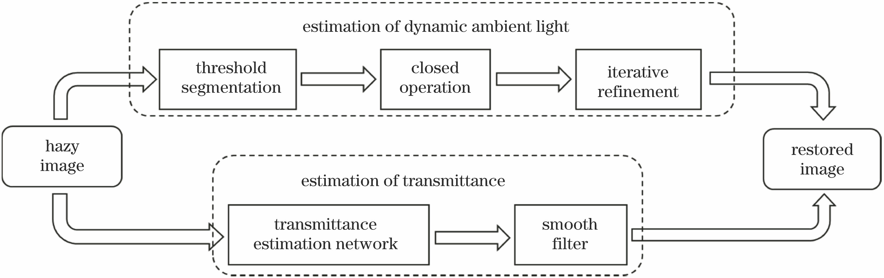
Fig. 1. Framework of the proposed algorithm

Download full size

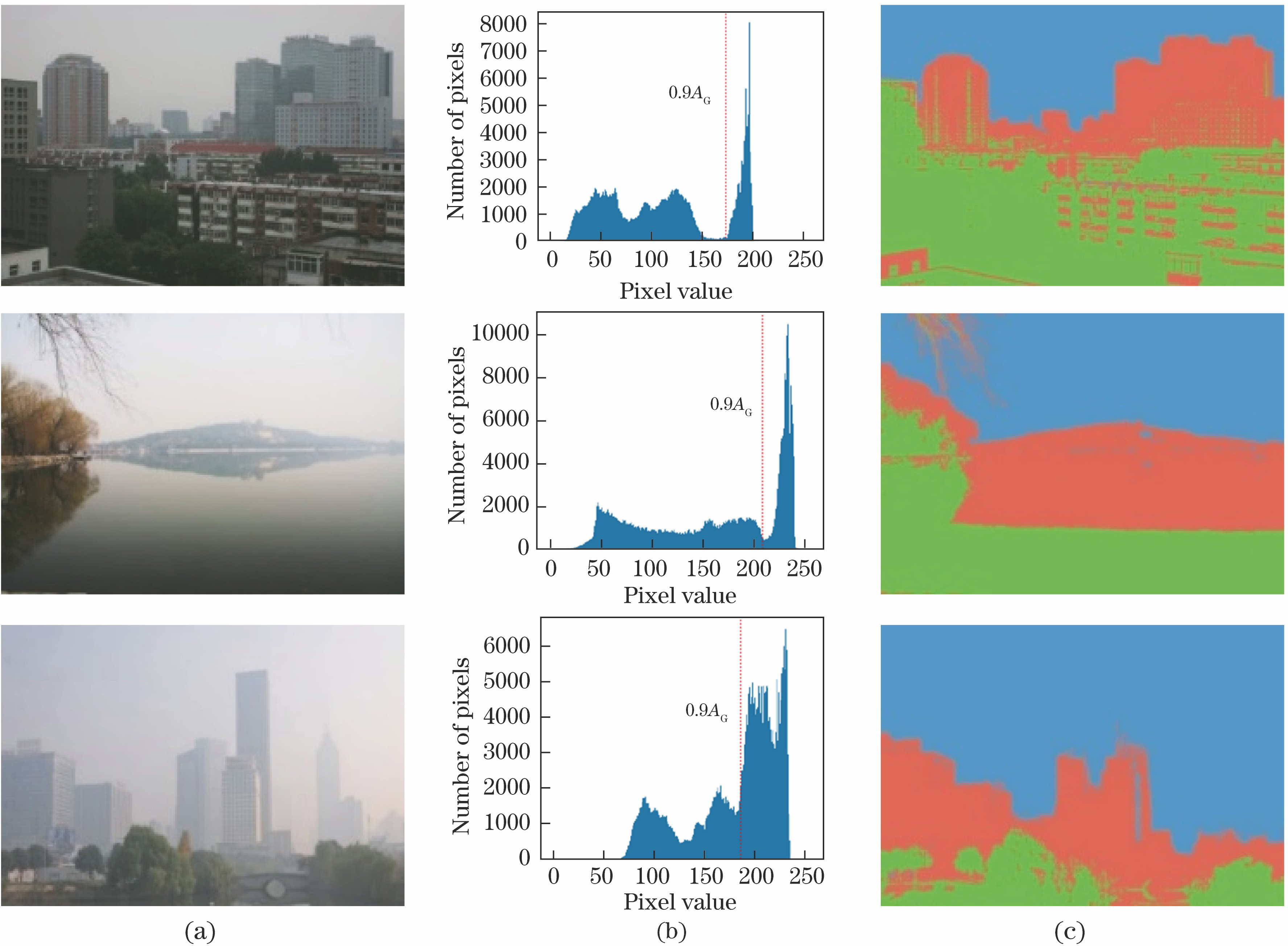
Fig. 2. Coarse segmentation of ambient light images. (a) Hazy images; (b) histograms of V channel; (c) regional segmentation

Download full size

Fig. 3. Dynamic ambient light. (a) Hazy images; (b) rough ambient light maps; (c) refined ambient light maps

Download full size

Fig. 4. Examples of training set. (a) Real hazy images; (b) transmittance images; (c) paired training samples

Download full size

Fig. 5. Structure of TEN

Download full size

Fig. 6. Estimation and refinement of transmittance. (a) Hazy images; (b) transmittance estimated by TEN; (c) refined transimittance

Download full size

Fig. 7. Comparison of transmittance estimation effects. (a) Hazy images; (b) transmittance estimated by TEN2; (c) transmittance estimated by TEN1; (d) restored results of TEN2; (e) restored results of TEN1

Download full size

Fig. 8. Restored effects of global and dynamic ambient light. (a) Hazy images; (b) results restored by global atmospheric light; (c) results restored by dynamic ambient light

Download full size

Fig. 9. Dehazing results of different algorithms. (a) Hazy images; (b) method in Ref. [4-5]; (c) method in Ref. [6]; (d) method in Ref. [9]; (e) method in Ref. [10]; (f) proposed algorithm

Download full size

Training set	Standard deviation	Average gradient	Information entropy	Edge intensity
Ref. [6]	60.21	8.22	7.21	59.26
Ref. [9]	59.23	8.05	7.22	58.07
Ref. [7]	62.59	8.17	7.22	58.80
Ref. [18]	64.02	9.55	7.21	69.03

Table 1. Comparison of average objective indexes of dehazing images using the trained network with different training sets

Algorithm	Standard deviation	Average gradient	Information entropy	Edge intensity
Method in Ref. [4-5]	45.12	7.82	7.02	57.07
Method in Ref. [6]	51.35	7.65	7.14	55.50
Method in Ref. [9]	51.41	7.13	7.16	51.34
Method in Ref. [10]	51.32	8.04	7.20	57.82
Proposed method	64.02	9.55	7.21	69.03

Table 2. Comparison of average objective indexes of dehazing images with different algorithms

Image	Algorithm	Standard deviation	Average gradient	Information entropy	Edge intensity
Img1	Method in Ref. [4-5]	52.95	7.47	7.40	58.53
	Method in Ref. [6]	61.70	7.49	7.34	59.37
	Method in Ref. [9]	66.51	6.95	7.19	55.70
	Method in Ref. [10]	62.45	7.27	7.34	58.09
	Proposed method	76.28	9.00	7.54	71.62
Img2	Method in Ref. [4-5]	45.33	13.02	7.47	89.47
	Method in Ref. [6]	49.40	11.29	7.33	76.85
	Method in Ref. [9]	37.43	8.90	7.09	62.69
	Method in Ref. [10]	57.02	13.05	7.53	88.99
	Proposed method	70.11	15.25	7.63	104.10
Img3	Method in Ref. [4-5]	55.74	12.98	7.41	86.35
	Method in Ref. [6]	55.60	12.96	7.61	86.28
	Method in Ref. [9]	52.08	10.85	7.52	74.17
	Method in Ref. [10]	67.54	14.61	7.62	97.78
	Proposed method	77.63	18.01	7.23	119.85
Img4	Method in Ref. [4-5]	49.30	17.69	7.54	119.87
	Method in Ref. [6]	49.96	15.82	7.56	107.62
	Method in Ref. [9]	56.78	15.93	7.60	106.44
	Method in Ref. [10]	59.89	18.47	7.75	120.96
	Proposed method	76.47	22.08	7.60	149.85
Img5	Method in Ref. [4-5]	49.67	9.81	7.27	65.23
	Method in Ref. [6]	49.98	10.22	7.29	67.33
	Method in Ref. [9]	50.89	9.40	7.29	65.60
	Method in Ref. [10]	54.45	9.89	7.24	69.11
	Proposed method	61.95	12.11	7.36	78.80
Img6	Method in Ref. [4-5]	33.07	5.11	6.82	35.96
	Method in Ref. [6]	51.43	5.45	7.35	38.38
	Method in Ref. [9]	59.43	4.70	7.57	34.38
	Method in Ref. [10]	50.14	5.03	7.40	36.77
	Proposed method	72.29	6.75	7.63	46.94

Table 3. Comparison of objective indicators of dehazing images with different algorithms

Jieping Liu, Yezhang Yang, Minyuan Chen, Lihong Ma. Image Dehazing Algorithm Based on Convolutional Neural Network and Dynamic Ambient Light[J]. Acta Optica Sinica, 2019, 39(11): 1110002

Download Citation

Set citation alerts for the article

Tools

Set citation alerts for the article

Save the article for my favorites

Paper Information