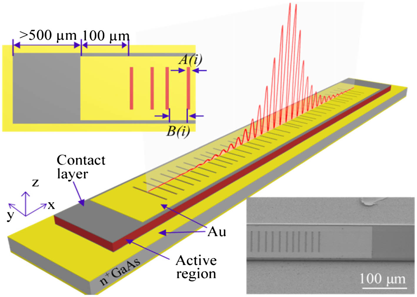
Fig. 1. Diagram of the THz QCL structure with a 1D disordered grating. Insets: top view of the device (top left), and scanning electron microscope (SEM) image of the fabricated QCL with disordered grating (bottom right); here, the aperture width is 3.5 μm and the disorder degree is 0.2.

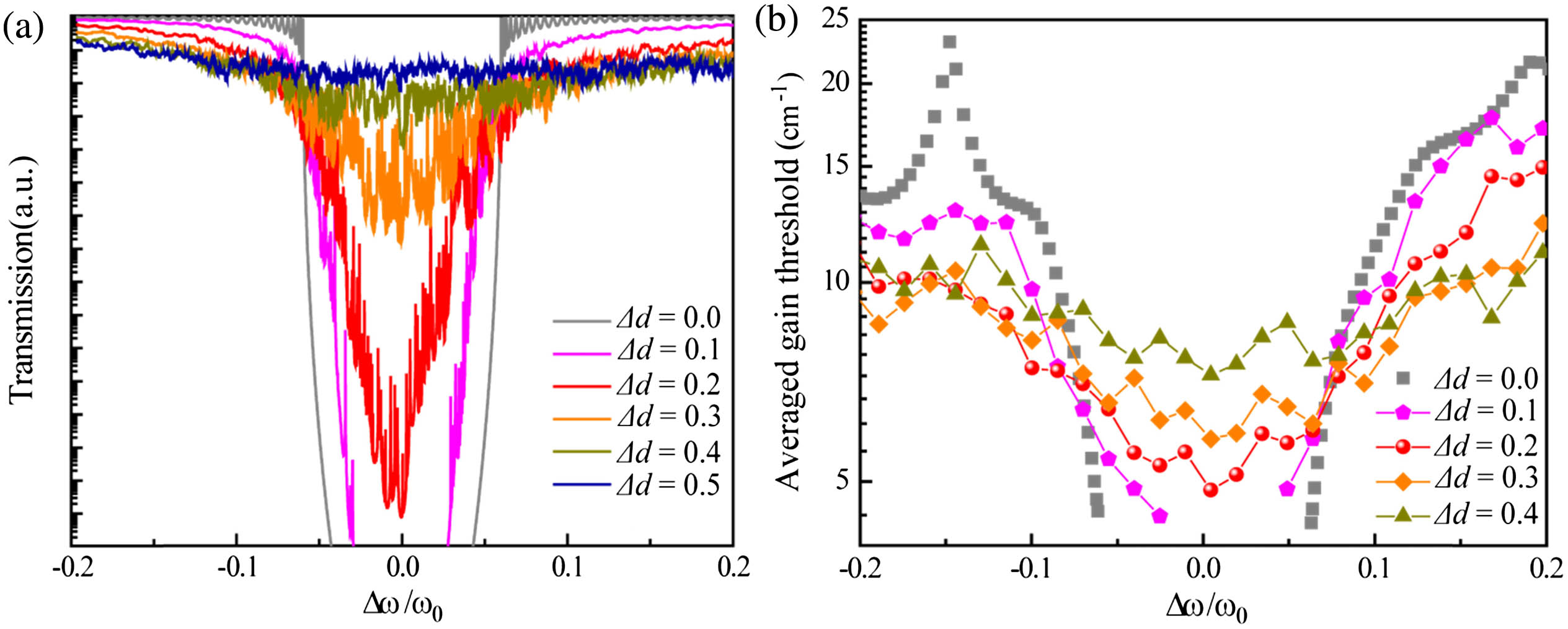
Fig. 2. (a) Ensemble-averaged transmission spectrum over 100 different configurations of the 1D disordered gratings for each degree of disorder. In the simulation, the 3D disordered waveguide structure was simplified to a 1D grating using an estimated refractive index contrast and without considering waveguide or material loss. (b) Ensemble-averaged gain threshold, calculated from 20 different configurations for each degree of disorder and taking the mean gain threshold at each frequency bin. The simulation was simplified to a 2D calculation of the structural cross sections where the x–z plane was considered, while the grating was assumed to be infinite in the y direction. For Δd=0, the peak at Δω/ω0=−0.15 is induced by resonance with the wire bonding areas. This resonance is disrupted and therefore disappears when disorder is introduced. The free carrier absorption losses of the active material were not considered.

Fig. 3. (a) LIV curves and (b) emission spectrum at 4.26 A for the fabricated 1D periodic QCL. (c) LIV curves and (d) emission spectra for the fabricated 1D disordered QCL with Δd=0.2. Emission spectra were measured at a heat-sink temperature of 10 K with a resolution of 0.2  cm−1. Aperture width of the devices is 3.5 μm.

Fig. 4. (a) Diagram showing two different sets of disordered gratings with disorder degree of Δd=0.2 fabricated on the same ridge, with the two lasers being pumped separately. (b) Emission spectra under different pumping conditions. Peaks are labelled by the frequency value in THz. (c) Calculated mode distributions (red curves) corresponding to four emission peaks when the “cold” laser was not pumped. The simulation was simplified to a 2D calculation of the structural cross sections where the x–z plane was considered, while the grating was assumed to be infinite in the y direction. For the cold laser, imag(nGaAs/AlGaAs)=−0.01i; while for the hot laser, imag(nGaAs/AlGaAs)=0.01i. Inset: field distribution snapshots of the top-view structure calculation (x–y plane within the active region, as shown in Fig. 1). The calculation results for cross section (red curves) and top view (field distribution snapshots) of the same structure agree well.

Fig. 5. Emission spectra of a 1D disordered QCL without (red curve) and with (violet dashed curve) partial covering by a copper sheet. The pumping current is 4.09 A. All the peaks are labelled by their frequency values in THz. The arrows are referred to in the text.

Table 1. Peak Frequencies (THz) and the Corresponding Lasing Threshold Currents (A) Corresponding to the Spectra in Fig. 3(d)