
Ziyang Chen, Fuqiang Li, Cibo Lou, "Statistical study on rogue waves in Gaussian light field in saturated nonlinear media," Chin. Opt. Lett. 20, 081901 (2022)
- Chinese Optics Letters
- Vol. 20, Issue 8, 081901 (2022)
Abstract
1. Introduction
Optical rogue waves (RWs) were first discovered, to the best of our knowledge, in nonlinear fiber supercontinuum experiments[
2. Experiment
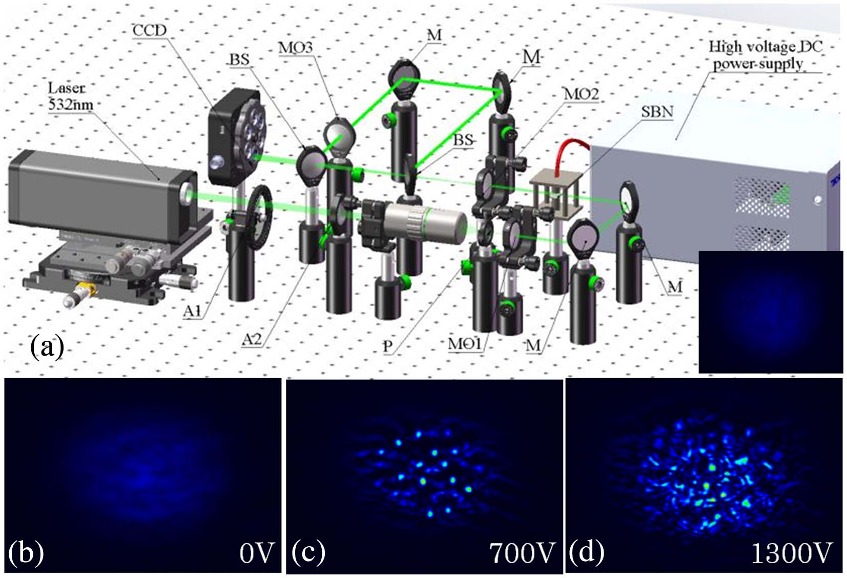
Therefore, we observe the phenomenon of wide GB splitting through experiments and numerical simulations to study the relationship between Gaussian MI and RWs and analyze the probability and spatial distribution of RWs. As shown in Fig. 1(a), we use an SBN crystal with a cross-sectional area of
![]()
Figure 1.(a) Experimental setup for observing RWs. Inset: input profile. (b)–(d) Output beam profiles for indicated voltages.
We change the NL to study the change in the probability of RWs in the phenomenon of filament separation. Without applying any voltage, as shown in Fig. 1(b), the outline of the GB propagating at 10 mm in the crystal is the same as the input profile. It can be seen that the input light propagates parallel to the z axis inside the crystal, and the input light is a non-uniform GB with lots of perturbations. The perturbation in GB is provided by intensity mask A2. The perturbation intensity is approximately 20% of the light intensity. These perturbations are very important to our experiments, and they lead directly to filamentous processes under nonlinear conditions.
Sign up for Chinese Optics Letters TOC. Get the latest issue of Chinese Optics Letters delivered right to you!Sign up now
Our experiments were performed by adjusting the voltage to control the NL of the crystal at a larger incident size. As shown in Figs. 1(b)–1(e), this allows light to be concentrated in very specific regions due to the initial non-homogeneous intensity distribution and MI, resulting in high-intensity spots. Since wire splitting is not obvious under low voltage, we set the following rules for the applied voltage: the voltage is increased from 350 V to 1300 V, each time increasing by 50 V, and the image of the exit surface is collected after the crystal modulation is stabilized.
By the standard of space strange waves[
![]()
Figure 2.Statistical chart of RWs probability with indicated voltage in experiments.
3. Simulation
To verify the experimental phenomenon and find out the main reason for the generation of RWs under GB, we carried out a numerical simulation on the RWs appearing on SBN crystals and GB and compared it with the results on PB. The propagation of incident light in SBN follows the NLSE[
In the above formula,
In the above formula,
We add a noise seed with a certain width and intensity to the formula, the size of which is related to the GB intensity at the corresponding position; the average value is zero, and the maximum value of the noise seed is 21% of the original GB amplitude at the corresponding position. The beam transmission in the SBN is obtained by the stepped beam propagation method[
We set the input width to be 300 µm, the propagation distance to be 10 mm, the lateral width of the crystal to be
![]()
Figure 3.(a) Scintillation index of the exit surface at different voltages. (b) Statistical probability plot of Gaussian RWs versus voltage in numerical simulation. Inset: probability distribution of AI under 700 V.
The voltage was increased from 300 to 1300 V in 50 V increments. In the case of random perturbation, each voltage was repeated 400 times. As shown in Fig. 3, it can be clearly seen that the variation trend of the RWs occurrence probability is consistent with the experimental results and is more detailed. The occurrence probability of RWs has a peak point, and the peak appears at the first highest point of the RWs probability fluctuation. In both experiments and simulations, this maximum value appears around 450 V. We have counted the intensity distribution of light filament. From the inset of Fig. 3(b), it can be clearly seen that there is a
It can be seen from Figs. 2 and 3(b) that the numerical simulation shows a distribution trend close to the experiment. In order to test whether this phenomenon is unique to GB itself, we numerically simulate the probability of RWs on a Gaussian amputation PB under the same conditions. As shown in Fig. 4, PB also has the statistical characteristics where the occurrence probability of RWs fluctuates with voltage, and the highest probability is located at the second peak after the occurrence of RWs. It can also be seen from Figs. 3(b) and 4 that the split light spots satisfy the long-tailed distribution statistically and meet the criterion of RWs.
![]()
Figure 4.Statistical probability plot of plane RWs with voltage in numerical simulation. Inset: probability distribution of ratio of emitted light intensity to Ie under 600 V.
This phenomenon is inconsistent with the traditional concept of RWs formation. To explain this phenomenon, we carried out numerical statistics on the maximum light intensity and wave number at different voltages. The statistical results are shown in the Fig. 5; when the propagation distance, light intensity, beam width, and perturbation range are fixed, RWs are more likely to appear at a specific voltage. At a suitable voltage, Gaussian light with corresponding width, intensity, and perturbation level is more likely to evolve to a high-intensity filament. Since the wave number decreases only slightly with increasing voltage, the number of high-intensity filaments directly determines the probability of RW occurrence. Voltage, or the magnitude of the NL, is also a parameter that has a complex effect on the RW phenomenon, rather than the simple positive correlation commonly thought.
![]()
Figure 5.Blue line shows the statistics of the maximum light intensity varying with voltage under GB. Red line shows the statistical graph of the wave number whose intensity is greater than Ie varies with voltage.
Although GB and PB have a similar trend in statistics, it can be seen that the probability of RWs appearing in the GB is much higher than that in the PB. To explain this result, we performed a numerical simulation of the propagation process under GB and PB. As shown in Fig. 6, compared with PB, the overall light intensity distribution trend of GB after splitting is basically the same as that at incidence, and the intensity at the middle position is significantly higher than that at the margin. The intensity difference caused by the initial distribution will cause a larger gap between the large peak wave and
![]()
Figure 6.(a)–(c) Light intensity distribution during GB propagation at different voltages. (d)–(f) Light intensity distribution during PB propagation at different voltages.
4. Supplementary Experiment
We use spatial frequency as the basis for judging the phenomenon of filament separation. As shown in Fig. 1(a), we added two beam splitters (BSs) to the original imaging system to image part of the light on the front focal plane of the Fourier lens MO3 [see Fig. 1(a)], so that the CCD is precisely on the Fourier plane. In this way, we get the spatial frequency of the back light of SBN. As shown in Figs. 7(a)–7(f), the discrete high-frequency components caused by RWs and low-frequency components caused by the PB background appear at the same time along with the filaments.
![]()
Figure 7.(a)–(c) Output beam profiles for indicated voltages. (d)–(f) Spatial spectra of output beams.
5. Conclusion
In summary, the formation mechanism of broad-GB excited RWs under saturation NL is much more complicated than generally thought. An increase in NL will cause the increase in average light intensity, so even with increasing dispersion, the odds of RWs still decrease. It is not simply reduced, but determined by the breathing behavior after the filaments separation. Statistically, the probability of occurrence of RWs excited by wide GB is much higher than that excited by PB. This is caused by the intensity gradient of GB itself. The weak light part of GB reduces the average light intensity after filament splitting. It can also be seen from Fig. 6 that the occurrence probability of waves with different propagation lengths and large amplitudes is not just positively correlated. We are designing an experiment that we hope to confirm it experimentally.
References
[1] D. R. Solli, C. Ropers, P. Koonath, B. Jalali. Optical rogue waves. Nature, 450, 1054(2007).
[2] A. Montina, U. Bortolozzo, S. Residori, F. T. Arecchi. Non-Gaussian statistics and extreme waves in a nonlinear optical cavity. Phys. Rev. Lett., 103, 173901(2009).
[3] D. Buccoliero, H. Steffensen, H. Ebendorff-Heidepriem, T. M. Monro, O. Bang. Midinfrared optical rogue waves in soft glass photonic crystal fiber. Opt. Express, 19, 17973(2011).
[4] A. Degasperis, S. Wabnitz, A. B. Aceves. Bragg grating rogue wave. Phys. Lett. A, 379, 1067(2015).
[5] J. He, S. Xu, K. Porseizan. N-order bright and dark rogue waves in a resonant erbium-doped fiber system. Phys. Rev. E, 86, 066603(2012).
[6] R. Gupta, C. N. Kumar, V. M. Vyas, P. K. Panigrahi. Manipulating rogue wave triplet in optical waveguides through tapering. Phys. Lett. A, 379, 314(2015).
[7] N. Akhmediev, A. Ankiewicz, M. Taki. Waves that appear from nowhere and disappear without a trace. Phys. Lett. A, 373, 675(2009).
[8] N. N. Akhmediev, V. I. Korneev. Modulation instability and periodic solutions of the nonlinear Schrödinger equation. Theor. Math. Phys., 69, 1089(1986).
[9] Y. C. Ma. The perturbed plane-wave solutions of the cubic Schrödinger equation. Stud. Appl. Math., 60, 43(1979).
[10] D. H. Peregrine. Water waves, nonlinear Schrödinger equations and their solutions. ANZIAM J., 25, 16(1983).
[11] N. Marsal, V. Caullet, D. Wolfersberger, M. Sciamanna. Spatial rogue waves in a photorefractive pattern-forming system. Opt. Lett., 39, 3690(2014).
[12] D. Pierangeli, F. D. Mei, C. Conti, A. J. Agranat, E. DelRe. Spatial rogue waves in photorefractive ferroelectrics. Phys. Rev. Lett., 115, 093901(2015).
[13] M. O. Ramírez, D. Jaque, L. E. Bausá, J. G. Solé, A. A. Kaminskii. Coherent light generation from a Nd: SBN nonlinear laser crystal through its ferroelectric phase transition. Phys. Rev. Lett., 95, 267401(2005).
[14] D. Pierangeli, F. D. Mei, G. D. Domenico, A. J. Agranat, C. Conti, E. DelRe. Turbulent transitions in optical wave propagation. Phys. Rev. Lett., 117, 183902(2016).
[15] D. Kip, M. Soljacic, M. Segev, E. Eugenieva, D. N. Christodoulides. Modulation instability and pattern formation in spatially incoherent light beams. Science, 290, 495(2000).
[16] C. C. Jeng, Y. Y. Lin, R. C. Hong, R. K. Lee. Optical pattern transitions from modulation to transverse instabilities in photorefractive crystals. Phys. Rev. Lett., 102, 153905(2009).
[17] A. Mathis, L. Froehly, S. Toenger, F. Dias, G. Genty, J. M. Dudley. Caustics and rogue waves in an optical sea. Sci. Rep., 5, 12822(2015).
[18] S. Lan, M. F. Shih, M. Segev. Self-trapping of one-dimensional and two-dimensional optical beams and induced waveguides in photorefractive KNbO3. Opt. Lett., 22, 1467(1997).
[19] C. Hermann-Avigliano, I. A. Salinas, D. A. Rivas, B. Real, A. Mančić, C. M. Cortés, A. Maluckov, R. A. Vicencio. Spatial rogue waves in photorefractive SBN crystals. Opt. Lett., 44, 2807(2019).
[20] R. Allio, D. Guzmán-Silva, C. Cantillano, L. Morales-Inostroza, D. Lopez-Gonzalez, S. Etcheverry, R. A. Vicencio, J. Armijo. Photorefractive writing and probing of anisotropic linear and non-linear lattices. J. Opt., 17, 025101(2014).
[21] F. Chen, M. Stepić, C. E. Rüter, D. Runde, D. Kip, V. Shandarov, O. Manela, M. Segev. Discrete diffraction and spatial gap solitons in photovoltaic LiNbO3 waveguide arrays. Opt. Express, 13, 4314(2005).


Set citation alerts for the article
Please enter your email address

© Copyright 2018-2021 | Chinese Laser Press. All Rights Reserved 沪ICP备15018463号-20