
Zewen He, Qiushi Zhuang, Huining Cao, Yu Xin. Focusing Through Scattering Medium Based on Memetic Algorithm[J]. Laser & Optoelectronics Progress, 2021, 58(24): 2429001
- Laser & Optoelectronics Progress
- Vol. 58, Issue 24, 2429001 (2021)
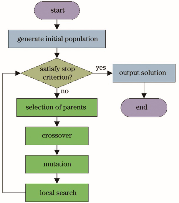
Fig. 1. Flow chart of the MA
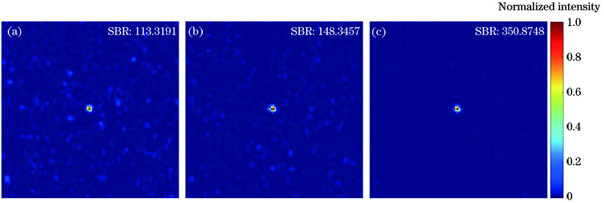
Fig. 2. Single-point focusing effect of three algorithms (simulation experiment). (a) GA; (b) PSO; (c) MA
Fig. 3. Variation curve of the single-point focus SBR of three algorithms with the number of iterations (simulation experiment)
Fig. 4. Schematic of the experimental setup
Fig. 5. Single-point focusing results of three algorithms (real environment). (a) GA; (b) PSO; (c) MA
Fig. 6. Variation curve of single-point focus SBR of three algorithms with the number of iterations (real environment)
Fig. 7. Multi-point focusing effect of pattern D. (a) Original image; (b) GA; (c) PSO; (d) MA
Fig. 8. Multi-point focusing effect of pattern H. (a) Original image; (b) GA; (c) PSO; (d) MA
Fig. 9. Multi-point focusing effect of pattern N. (a) Original image; (b) GA; (c) PSO; (d) MA
Fig. 10. Multi-point focusing effect of pattern T. (a) Original image; (b) GA; (c) PSO; (d) MA
|
Table 1. Running time of three algorithms (simulation experiment) unit: s
|
Table 2. Running time of three algorithms (real environment) unit: s
|
Table 3. Correlation coefficients of three algorithm multi-point focusing maps

Set citation alerts for the article
Please enter your email address
© Copyright 2018-2021 | Chinese Laser Press. All Rights Reserved 沪ICP备15018463号-20