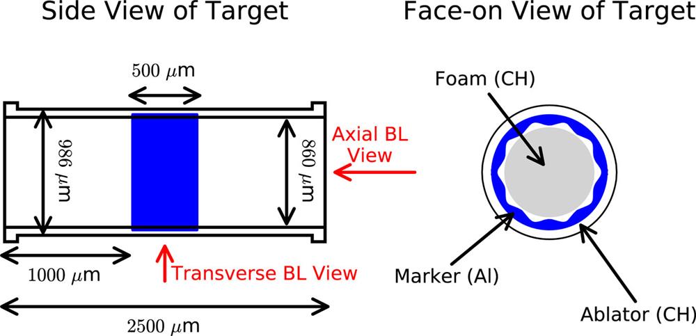
Fig. 1. Schematic layout of target for OMEGA. The imaging axes for the transverse and axial backlighters are also shown.

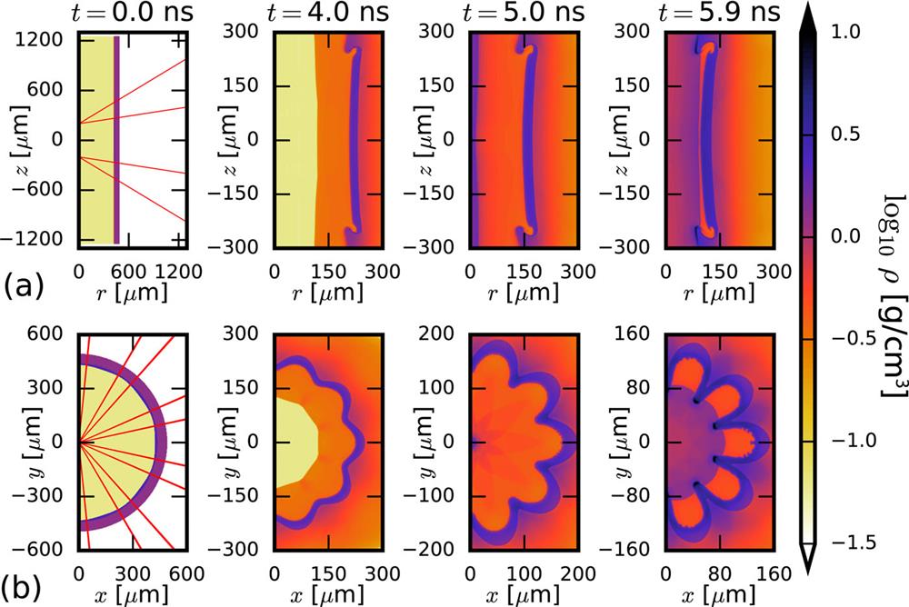
Fig. 2. Simulated density profiles from (a) r–z computation and (b) r–θ computation (m = 10, a₀ = 3 µm initially).

Fig. 3. (a) Side-on synthetic radiographs from the r–z simulation shown in Fig. 2(a). (b) Down-axis synthetic radiographs incorporating the r–θ results shown in Fig. 2(b).

Fig. 4. A comparison of synthetic radiographs looking down the cylinder axis. (a) Results from an r–θ simulation with no initial perturbation are used over the 500 µm marker extent. (b) r–z simulation results are used over the entire axial extent.

Fig. 5. Inner marker radius vs time for 1D, 2D r–θ, and 2D r–z simulations.

Fig. 6. (a) Radius vs time for the inner surface of the cylinder with subsequent calculations of velocity and acceleration of the interface. (b) Density on each side of the inner surface interface and the corresponding Atwood number. (c) Predicted amplitudes for mode 10 growth using the linear theory of Ref. 38 and a modified nonlinear theory of Ref. 39, which predicts different growth rates for bubbles and spikes.

Fig. 7. Comparison of 2D xRAGE simulations of perturbation growth with the linear theory of Ref. 38 and the weakly nonlinear buoyancy-drag (BD) model of Ref. 39 for (a) the m = 4 mode at 4 µm initial amplitude and (b) the m = 10 mode at 3 µm initial amplitude.

Fig. 8. (a) Radius of inner surface of marker band vs time for various laser coupling efficiencies. (b) Calculated linear growth factor vs time for modes 4 and 10 for the corresponding coupling efficiencies.

Fig. 9. (a) Pie diagram showing the radial hydrodynamic scaling of the OMEGA cylinder design (the void between CH foam and Al marker is not modeled here). (b) Schematic of the NIF-scale target.

Fig. 10. Laser power deposition (left column) and mass density (four right columns) at several different times, showing marker bowing for NIF-scale r–z computations with an 800 µm long marker. Laser beams are displaced axially by (a) 1000 µm, (b) 1025 µm, and (c) 1050 µm.

Fig. 11. Results from 1D simulations of the NIF-scale target using a 3 ns square pulse: (a) 1.0× hydro-scaled drive and 60 mg/cm³ foam fill; (b) 1.0× hydro-scaled drive and 30 mg/cm³ foam fill; (c) 1.5× hydro-scaled drive and 30 mg/cm³ foam fill; (d) 2.0× hydro-scaled drive and 30 mg/cm³ foam fill; (e) 1.0× hydro-scaled drive and 10 mg/cm³ deuterium fill; (f) 1.0× hydro-scaled drive and 5 mg/cm³ deuterium fill.