1State Key Laboratory of Integrated Service Networks, State Key Discipline Laboratory of Wide Bandgap Semiconductor Technology, Xidian University, Xi’an 710071, China
2Yongjiang Laboratory, Ningbo 315202, China
3Key Laboratory of Intelligent Optical Sensing and Manipulation, Ministry of Education, the National Laboratory of Solid State Microstructures, the College of Engineering and Applied Sciences, Institute of Optical Communication Engineering, Nanjing University, Nanjing 210023, China
Spiking neural networks (SNNs) utilize brain-like spatiotemporal spike encoding for simulating brain functions. Photonic SNN offers an ultrahigh speed and power efficiency platform for implementing high-performance neuromorphic computing. Here, we proposed a multi-synaptic photonic SNN, combining the modified remote supervised learning with delay-weight co-training to achieve pattern classification. The impact of multi-synaptic connections and the robustness of the network were investigated through numerical simulations. In addition, the collaborative computing of algorithm and hardware was demonstrated based on a fabricated integrated distributed feedback laser with a saturable absorber (DFB-SA), where 10 different noisy digital patterns were successfully classified. A functional photonic SNN that far exceeds the scale limit of hardware integration was achieved based on time-division multiplexing, demonstrating the capability of hardware-algorithm co-computation.
By drawing on the structure and information processing of the nervous system, the new paradigm of neuromorphic computing with non-von Neumann architectures has driven further development of low-power and low-latency computing systems. Nowadays, neuromorphic learning is mostly software-based and inherently limited by the von Neumann bottleneck. Spiking neural networks (SNNs), known as the third-generation neural networks, are considered to be the most bio-realistic1, 2. SNNs employ spatiotemporal coding, and exploit low-power characteristics due to sparse spike transmission3-6. The SNN architecture mainly consists of three parts, the neural computational units, synaptic connections, and learning rules.
As the most important element in neural networks, theoretical models and hardware emulations of neurons have received extensive attention in both the electrical and optical domains. However, due to the complex biological mechanisms of neurons, the cells and synapses of neurons are usually treated separately as nonlinear computational units and tunable connections in artificial neural networks.
In the field of microelectronics, neurons based on complementary metal-oxide-semiconductor technology memristor arrays7-10, transistors11, 12 and VLSIs13 have achieved tremendous improvements. While such microelectronic neurons can exceed biological time scales, they are subject to fundamental bandwidth fan-in trade-offs and suffer from deficiencies in energy efficiency, speed, etc.14. Due to the high speed, high bandwidth, and achievable low crosstalk of optical platforms, optical computing has attracted lots of attention15-21, including linear computing such as matrix multiplication15, 16, all optical logic gate17, photonic synapses and neurons21, etc. Photonic neurons have received increasing attention as a promising candidate for artificial neurons, and a great deal of effort has been devoted to the exploration of photonic devices.
To date, significant efforts have been dedicated to emulating photonic spiking neurons. The basic neuron-like dynamics such as spiking, integration, threshold behavior and relative refractory period have been observed in various types of lasers22, including ring lasers23, vertical cavity surface emitting semiconductor lasers (with a saturable absorber)24-27, distributed feedback semiconductor (DFB) lasers, and DFB lasers with a saturable absorber (DFB-SA)28-30, Fabry-Pérot lasers with a saturable absorber (FP-SA)31, semiconductor micropillar lasers32, etc. Based on the nonlinear computing of photonic spiking neurons, photonic SNNs have been implemented for simple pattern recognition31, 33 and sound direction detection28 with the help of algorithms. In photonic SNNs, the basic feed-forward structure is the most adopted. However, in biological nervous systems, the neural coupling is usually not unidirectional and unique. There may be multiple coupling paths between two neurons with different efficacies and delays34-37. However, there is not much attention paid on the impact of multiple connections in optical computing.
Here, we present a supervised learning scheme in temporal encoding photonic SNN for pattern classification with the introduction of multisynapse couplings and provide experimental demonstration via a fabricated DFB-SA chip. The main contributions of this work lie in: Firstly, we introduce multisynapse couplings in photonic SNN for the first time, where multiple coupling paths between two neurons with different efficacies and delays are considered. Then, the digit pattern classification is performed numerically to demonstrate the improvements of network performance. Finally, the collaborative learning of algorithms and hardware devices is further demonstrated experimentally based on a single fabricated DFB-SA chip via using time-multiplexed spike encoding.
Methods
Experimental setup
The multi-synaptic connection in the biological neural network is illustrated in Fig. 1(a), where synaptic connections from presynaptic neurons are distributed in the dendritic tree of the postsynaptic neuron36. The soma in the postsynaptic neuron integrates the received signals and converts the input signals into spike forms. The coupling delay and efficacy of synapses differ.
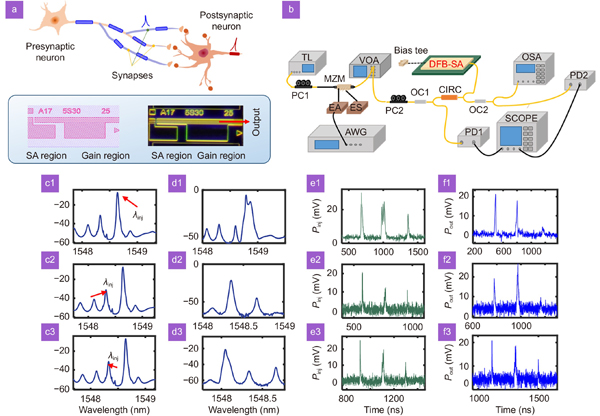
Figure 1.(a) The geometry of multi-synaptic connections. (b) The experimental setup. The optical path is denoted by yellow, and the electrical path is black. The GDS file and chip micrograph of the DFB-SA neuron chip. (c1–c3) The optical spectrum of free-running DFB-SA, marked with different injection wavelengths. (d1–d3) The optical spectrum of DFB-SA with external optical injection corresponding to (c1–c3). (e1–e3) and (f1–f3) The input pattern and the corresponding output.
In the experiment, we adopted a fabricated DFB-SA chip to perform the nonlinear activations of the postsynaptic neuron. The experimental setup used for verifying the nonlinear computing based on the DFB-SA spiking neuron is presented in Fig. 1(b). The GDS profile and chip micrograph of the DFB-SA are illustrated respectively. The system mainly consists of the core computing chip and the peripheral circuit for modulation and control. In the experiment, the gain region of the DFB-SA is driven by a current source, denoted as the gain current IG, while the SA region is reversely driven by a voltage source, denoted as VSA. A tunable laser (TL; AQ2200-136 TLS module, Yokogawa) is used to provide the optical carrier with a center wavelength of λinj. The input spike sequence is firstly written into the arbitrary waveform generator (AWG; AWG70001A, Tektronix) with a sampling rate of 10.5 GHz, then modulated into the optical carrier through a Mach-Zehnder modulator (MZM, Fujitsu FTM7928FB). After power control with a variable optical attenuator (VOA), the modulated signal is injected into the DFB-SA via a three-port optical circulator (CIRC). The modulated optical signal and the output of the DFB-SA are converted to electrical signals by photodetectors (PDs, Agilent HP11982A), recorded and observed by an oscilloscope (OSC, Keysight DSOV334A). The optical spectrum of the DFB-SA is recorded and analyzed by an optical spectrum analyzer (OSA, Advantest Q8384).
The two-section structure of DFB-SA allows it to simulate the basic dynamics of leaky-integrate and fire (LIF) neurons. We firstly demonstrate the integrattion and threshold behaviors of the photonic spiking neuron. Different injection methods are compared. We consider coherent injection when the injection wavelength λinj is close to the dominate mode, and incoherent injection when λinj is away from the dominant mode. Figure 1(c1–c3) show the optical spectrum of free-running DFB-SA. The external optical signal is injected into the dominate mode (λinj=1548.64 nm), the first side mode (λinj=1548.33 nm) and the second side mode (λinj= 1548.11 nm), respectively. The corresponding optical spectrum with external optical injection is presented in Fig. 1(d1–d3). The input pattern is encoded into several spikes with different amplitude and distance (Fig. 1(e1–e3)). The first high spike is used to demonstrate the spiking dynamics of DFB-SA. The second weak spike is actually a cluster of several very close spikes, for the revealing of integration behavior. The third single weak spike is used for threshold demonstration. The corresponding output pattern is shown in Fig. 1(f1–f3). We can observe that when injected into the dominate mode and the first side mode, the single weak pulse causes no obvious spike generation, however a cluster of spikes with similar amplitude can make the neuron generate a clear spike that is similar to the spike generated via a single high pulse, demonstrating the integration and threshold dynamics of the photonic spiking neurons. However, when injected into the second side mode which is more far from the dominate mode, the neuron responds almost consistent with the input. Hence, we adopt coherent injection to perform pattern classification in the following.
Algorithms comparison
To accomplish efficient hardware-based computation, the basic architecture for temporal-coding supervised learning in SNN is introduced here, which consists of 5 parts, including the spatio-temporal encoding part, the input layer, the reconfigurable weight and delay arrays, the output layer, and the control unit. As shown in Fig. 2, in the encoding part, all input features are encoded into rectangular pulses, with the central timing carrying the specific feature. The pulse width and strength are properly selected to stimulate a single spike in the photonic spiking neuron of the input layer. The optical spikes generated from the input layer are then transmitted into the output layer, delayed and weighted separately via the delay and the weight arrays. The feedforward signals are received and activated via the output neuron. If the received inputs raise the carrier density of the output laser neuron above the threshold, which is also determined by the bias current of the gain region, a spike is generated, otherwise, the output neuron remains silent.
Figure 2.The basic structure for supervised learning of photonic SNNs with temporal coding.
The output spike timing and the input spike timing are detected in the control unit. In accordance with the algorithm, the weight and delay arrays are adjusted based on the calculated updates. In photonic SNNs, typically only online inference is conducted due to the challenges associated with controlling and storing optical signals. Once the weights and time delays are trained, they are configured into the network, enabling high-speed inference calculations at the velocity of light.
Here, we employed multi-synaptic connections in photonic SNNs to achieve 0~9 digit pattern classification. The processing is shown in Fig. 3(a). Each digit consists of a 20×20 pixel matrix, resulting in a 400-dimensional feature vector. Due to the relative simplicity of the task, the 400-dimensional input vectors were first reduced to 9 dimensions using principal component analysis in order to reduce the computational effort. Subsequently, the reduced input vector was transformed into rectangular spikes with distinct central timings based on the corresponding feature values, as illustrated in Fig. 2. After temporal encoding, the features were fed into the SNN. Each input neuron was connected to an output neuron through multiple synapses Nsyn, each possessing a different weight and time delay. Because there were multiple output neurons, the outputs of the neurons were encoded according to a set of orthogonal unit vectors, akin to the one-hot label. The dimension of the vector corresponds to the number of categories that need to be classified. For a neural network with input dimension Ni and output dimension No, when the k-th class sample (k=1,…,K; K=No) is fed in, the target vector is defined as tdk·ek, where ek denotes the k-th set of unit vectors. Consequently, the input of the k-th class samples is expected to elicit an active response from the k-th output neuron, while the other output neurons remain inactive, as illustrated in Fig. 3(b). In this task, the network size is determined by the input feature dimension and categories, namely, Ni =9, No =10.
Figure 3.(a) The process of digit pattern recognition based on a multi-synaptic photonic spiking neural network. (b) The output classification. (c) The basic principle for temporal coding SNN. (d) The STDP rule. (e) The mean distance of 4 different training methods with different Nsyn.
Predictably, multi-synaptic coupling enables robust information afference in a network. In the case that some pathways are disrupted, information can still be delivered via alternative ways. In addition, different coupling efficiencies and delays introduce noise in the network, which can prevent overfitting and to some extent improve the performance of the system.
In the following, to verify the role of multi-synaptic structures in pattern recognition tasks, we compare several common algorithms for temporal-coding feed-forward SNN training, including the well-known remote supervised method (ReSuMe)38, 39, Tempotron31, 40, and delay-weight combined ReSuMe (DW-ReSuMe)41-43. The principle for training a temporal coding SNN is displayed in Fig. 1(c). The weight is updated based on the difference of input spiking timing ti, the output spiking timing to, or the peak timing tmax if no spike is generated according to different algorithms. The optical spiking timing-dependent plasticity (STDP)39, 43 is combined to replace the kernel function. The traditional back-propagation method is also considered to provide a baseline.
To quantitatively describe the degree of convergence of the training process, we define Distance as the average of the differences between the targets assigned to all the output neurons and their actual behaviors for all input samples:
where k=1,…, K denotes the index of pattern categories, and j=1,…, No is the index of output neurons. describes the distance between the target assigned to the j-th output neuron when the k-th category is input, is the corresponding target spike number which is 0 when the neuron is expected to be silent, and is the actual output spike number. The average distance will be 0 when all the output neurons emit spikes according to their targets. For the BP method, the Distance can be calculated equivalently as the number of misclassified samples.
During the training process, the parameters of each synapse are adjusted independently according to the algorithm. Note the difference in the dimension of output neurons, when the target neuron is expected to generate a spike, the other neurons need to be silent. The results are given in Fig. 3(e). From where we can observe that with increasing Nsyn, the Distance of the network tends to be lower. When Nsyn=1, only the Distance calculated with DW-ReSuMe could converge to 0, indicating the highest calculation efficiency for simple pattern learning. We also test these methods based on a much more complex dataset MNIST. For each categories of hand-written digits, we randomly chose 20 samples from the training set and 10 samples from the test set. The selected dataset is further down-sampled via PCA to decrease the input dimension from 784 to 20. Moreover, to provide a baseline performance of the selected dataset, the convolutional neural network (CNN) and traditional artificial neural network (ANN) are also considered. 16 kernels with size 2×2 are used, so the input size of the fully connection layer is 28×28×16. The results are given in Table 1. It can be seen that in CNN with a single convolution and pooling layer, the mean accuracy could reach 80%. Then, the down sampled features are trained with 4 algorithms in the same network structure, and different numbers of synapses are compared. Not surprisingly, the ANN provide the best performance when Nsyn=3, reaching 60.67%. As for the temporal coding SNN algorithm, the DW-ReSuMe still performs better than ReSuMe and Tempotron. Overall, with multiple synapses, the mean accuracy increases for all methods.
Algorithm
Network size
Nsyn=1
Nsyn=2
Nsyn=3
Tempotron
20×10
(25.71±2.43)%
(30.4±3.51)%
(34.80±2.68)%
ReSuMe
20×10
(19.4±2.19)%
(27.75±5.56)%
(29.60±4.10)%
DL-ReSuMe
20×10
(37±7.78)%
(42.80±1.30)%
(47.20±2.39)%
ANN-BP
20×10
(54.60±7.13)%
(56.67±5.28)%
(60.67±3.14)%
CNN-BP
(784×16)×10
(79.4±1.52)%
/
Table 1. Accuracy of MNIST classification based on different models with different Nsyn.
In the previous section, it is demonstrated that in temporal coding SNN, the DW-ReSuMe performs well in comparison with other well-known methods. In this part, the DW-ReSuMe is adopted for further analysis. The classification of 0~9 digit patterns shown in Fig. 4 is performed based on the proposed network structure in conjunction with the modified DW-ReSuMe algorithm. Here, triple-synaptic connections are considered. The target timing for all 10 patterns is set to td=23 ns, whereas for neurons not expected to generate spikes, the corresponding target is set to the maximum simulation time T, where T = 40 ns. Figure 4 further illustrates the training process for all 10 output neurons when exposed to different input patterns. The rows in the figure indicate different output neurons and the columns correspond to different input patterns. It is evident that after several training epochs, all the output neurons produce a single spike at around 23 ns only when the corresponding category is input, while the other neurons remain resting.
Figure 4.The output spike timing of all 10 output neurons (the row) at the input of all 10 patterns (the column) when Nsyn=3.
Then, we trained the neural network with varying numbers of synaptic connections to investigate the effect of multi-synapses on the network performance. The results are presented in Fig. 5(a). As can be seen, when there is only one synapse, the training process is not stable, and the error distance fails to converge to 0. However, when two synapses are present, the distance converges to 0 after approximately 168 training cycles. Similarly, with three synapses, the error distance converges at the 214th training cycle. It is worth noting that the presence of three synapses introduces more learning parameters, making the network training more complex and resulting in a larger initial error. Therefore, it is not necessary to use as many synapses as possible to enhance network performance. Instead, a trade-off should be made between performance and training efficiency.
Figure 5.(a) The converged Distance with 1, 2, and 3 synapses, respectively. (b1–b2) Normalized weights for each of the two sets of synapses after convergence. (c1–c2) Normalized delays for each of the two sets of synapses after convergence. (d1) The converged Distance in the parameter space of weight mismatch and delay mismatch and (d2) projection of the contour with Distance=1.
For this task, the network performs best when Nsyn=2. In the following, we consider the case when Nsyn=2 for further analysis. Figure 5(b1–b2) and 5(c1–c2) present the weights and delays of the two sets of synapses after training convergence, noting that the initial values of weight and time delay for all synapses are uniform. It can be observed that the weights of the two groups of synapses change slightly compared to the change in delays, indicating that delay is a critical parameter in the temporal coding learning method. Besides, as the parameters of the two groups of synapses were trained independently, the final results also differed significantly.
Furthermore, we conducted an analysis to assess the robustness of the network by investigating the impact of deviations in weight and delay configurations on its performance. To quantitatively characterize the introduced parameter mismatches, the weights were normalized to 1 and the time delays were normalized to 1 ns. Gaussian noise with intensities ranging from 0 to 0.5 for weights and from 0 to 0.1 ns for time delays was then added. The calculation was repeated five times to obtain an average result, as depicted in Fig. 5(d1). The solid blue line in Fig. 5(d2) represents a contour projection with a Distance value of 1. Within the contour, the average distance is below 1, indicating the range of convergence. Notably, the network demonstrates low sensitivity to weight mismatches, but exhibits considerable sensitivity to deviations in time delays. A relative mismatch degree greater than 0.01 in time delays can lead to a significant decline in performance.
Experimental results and discussion
In the collaborative implementation of algorithms and hardware, input patterns with a delay noise of 0.01 and weight noise of 0 are selected. As can be seen from Fig. 5(d2), this condition corresponds to the boundary of convergence. Notice that the multi-synaptic network is essentially equivalent to feeding the same feature through multiple monosynaptic input neurons. After training convergence, for each sample, the input feature is first delayed and weighted via the trained weights and delays, then summated to form a single spike train, which represents exactly the input signals received by the single postsynaptic neuron. The spike sequence written into AWG is the delayed and weighted sum of all encoded features. Based on the DFB-SA chip, the outputs of all POST neurons are observed simultaneously using the time-division multiplexing method, as illustrated in detail in Fig. 6.
Figure 6.(a1–j1) The input spike patterns for all the 10 output neurons. (a2–j2) The correlated outputs of DFB-SA. (k1) The output spike interval for all 10 output neurons of 20 experiment trials. (k2) The output spike power for all 10 output neurons of 20 experiment trials.
Figure 6(a1–j1) present the input encoding sequences for all the 10 input patterns, with each cycle containing 10 spike clusters representing the cumulative input signal received by each of the 10 output neurons. Each cluster comprises 18 spikes of varying intensities, representing the input signals afferent from the 9 input neurons each with 2 synapses. The corresponding output sequences from DFB-SA are shown in Fig. 6(a2–j2). Two cycles of the output patterns are shown in each subplot. For each input pattern, a spike can be elicited in the corresponding output neuron, while the rest of the neurons produce only low-amplitude perturbations, which are consistent with the simulation results.
To analyze the stability of the experimental results, we repeated each set of experiments 20 times and recorded the timing and amplitude of the output spikes. Figure 6(k1) illustrates the spike time interval of the output spike train across 20 experiments for all 10 patterns. We can see that in most cases, the spike interval is quite stable, demonstrating the stability of the photonic spiking neuron. However, for pattern 1 and pattern 8, the output spike is not stable because of the introduced noise as discussed earlier. It should be noted that working within the convergence region of parameter mismatches yields more stable results. Likewise, the spike amplitudes of the output spike trains across the 20 experiments for all 10 patterns are depicted in Fig. 6(k2). It can be observed that, compared to the spike timing intervals, the spike amplitudes display greater fluctuations. The amplitude fluctuation poses a problem of threshold selection to determine whether a spike is generated, which is less crucial in the inference of photonic SNN with temporal coding since information is carried in the specific timing of spikes.
Finally, the power consumption of the DFB-SA laser neuron is estimated. All the peripheral circuits are neglected, and we only focus on the power consumed by the DFB-SA for nonlinear computing. The power consumption can be calculated as the power difference of the modulated signals Pinj1 =31.09 μW (which is able to trigger a single spike) and the power before modulation Pinj2 =30.53 μW. That is to say, the power consumption of the nonlinear computing in DFB-SA is about 0.36 μW, which is comparable with the result obtained by an FP-SA31.
Conclusions
In this work, we proposed the use of multi-synaptic connectivity in photonic SNN with the modified ReSuMe algorithms based on delayed-weight co-training. We identified 0~9 digit patterns through numerical simulations and experiments. By investigating the effect of different numbers of synaptic couplings between input and output neurons, we found that multiple connections could effectively improve network performance. We also analyzed the robustness of the network by assessing the convergence of the network for different degrees of configuration errors in weights and delays. Finally, the collaborative computing of algorithm and hardware was implemented based on a single DFB-SA chip using a time-multiplexing approach. This work demonstrates efficient learning in photonic SNN via introducing multiple synapses, which is helpful in the future application of optical computing.
Acknowledgements
We are grateful for financial supports from the National Key Research and Development Program of China (Nos. 2021YFB2801900, 2021YFB2801901, 2021YFB2801902, 2021YFB2801903, 2021YFB2801904), the National Outstanding Youth Science Fund Project of National Natural Science Foundation of China (No. 62022062), the National Natural Science Foundation of China (No. 61974177) and the Fundamental Research Funds for the Central Universities (No. QTZX23041).
The authors declare no competing financial interests.
[2] N Rathi, I Chakraborty, A Kosta, A Sengupta, A Ankit et al. Exploring neuromorphic computing based on spiking neural networks: algorithms to hardware. ACM Comput Surv, 55, 243(2023).
[4] F Ponulak, A Kasinski. Introduction to spiking neural networks: information processing, learning and applications. Acta Neurobiol Exp, 71, 409-433(2011).
[18] CR Huang, VJ Sorger, M Miscuglio, M Al-Qadasi, A Mukherjee et al. Prospects and applications of photonic neural networks. Adv Phys:X, 7, 1981155(2022).
[19] JQ Gu, CH Feng, HQ Zhu, RT Chen, DZ Pan. Light in AI: toward efficient neurocomputing with optical neural networks—a tutorial. IEEE Trans Circuits Syst II:Express Briefs, 69, 2581-2585(2022).
[25] SY Xiang, H Zhang, XX Guo, JF Li, AJ Wen et al. Cascadable neuron-like spiking dynamics in coupled VCSELs subject to orthogonally polarized optical pulse injection. IEEE J Sel Top Quantum Electron, 23, 1700207(2017).
[43] SY Xiang, JK Gong, YH Zhang, XX Guo, YN Han et al. Numerical implementation of wavelength-dependent photonic spike timing dependent plasticity based on VCSOA. IEEE J Quantum Electron, 54, 8100107(2018).