High-precision algorithm for restoration of spectral imaging based on joint solution of double sparse domains

Shi-Jie LIU; Chun-Lai LI; Rui XU; Guo-Liang TANG; Bing WU; Yan XU; Jian-Yu WANG

doi:10.11972/j.issn.1001-9014.2021.05.016

Journals >Journal of Infrared and Millimeter Waves >Volume 40 >Issue 5 >Page 685 > Article

Journal of Infrared and Millimeter Waves
Vol. 40, Issue 5, 685 (2021)

High-precision algorithm for restoration of spectral imaging based on joint solution of double sparse domains

Shi-Jie LIU^1、2, Chun-Lai LI^1、*, Rui XU¹, Guo-Liang TANG^1、2, Bing WU^1、2, Yan XU^1、2、4, and Jian-Yu WANG^{1、2、3、**}

Author Affiliations

¹Key Laboratory of Space Active Opto-Electronics Technology，Shanghai Institute of Technical Physics，Chinese Academy of Sciences，Shanghai 200083，China

²University of Chinese Academy of Sciences，Beijing 100049，China

³Hangzhou Institute for Advanced Study，University of Chinese Academy of Sciences，Hangzhou，310024China

⁴School of Information Science&Techno1ogy，ShanghaiTech University，Shanghai 200020，China

show less

DOI: 10.11972/j.issn.1001-9014.2021.05.016 Cite this Article

Shi-Jie LIU, Chun-Lai LI, Rui XU, Guo-Liang TANG, Bing WU, Yan XU, Jian-Yu WANG. High-precision algorithm for restoration of spectral imaging based on joint solution of double sparse domains[J]. Journal of Infrared and Millimeter Waves, 2021, 40(5): 685 Copy Citation Text

show less

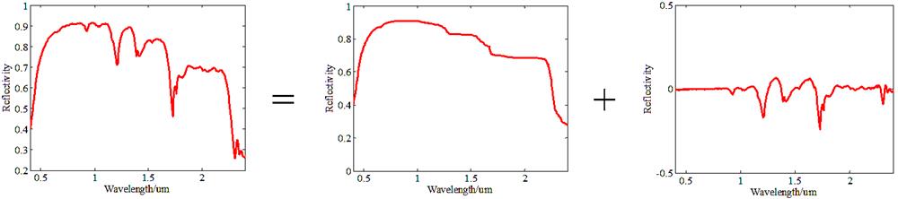
Fig. 1. Spectrum data can be divided into contour and details

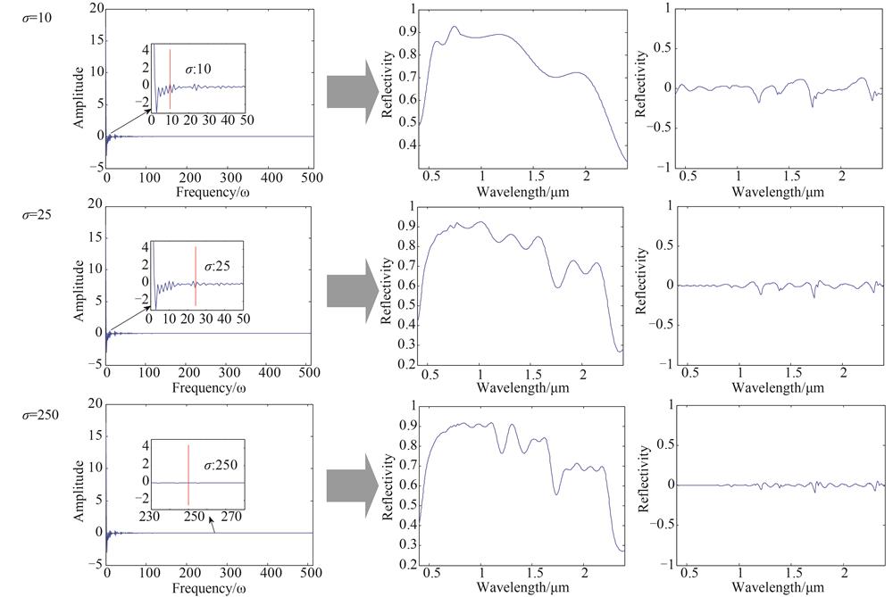
Download full size | View in the Article

Fig. 2. igh and low frequency distribution of corresponding signals when σ is 10，25，250

Download full size | View in the Article

Fig. 3. Recovery results of different sampling rates under different sparsity constraints (a) Sampling rate: 40%, σ: 10, (b) Sampling rate: 40%, σ: 25, (c) Sampling rate: 40%, σ: 250,(d) Sampling rate: 80%, σ: 10, (e) Sampling rate: 80%, σ: 25, (f) Sampling rate: 80%, σ: 250

Download full size | View in the Article

Fig. 4. Test results on 500 samples (a) (b): Comparison of recovery accuracy at different sampling rates (σ: 15) ,(c) (d):σ’s impact on recovery accuracy (Sampling rate: 40%)

Download full size | View in the Article

Fig. 5. Information distribution of carnauba wax spectrum corresponding to different sparse transforms（a）Distribution of different sparse transform coefficients，（b）：Distribution during signal reconstruction at σ=10，（c）Distribution during signal reconstruction at σ=100

Download full size | View in the Article

Fig. 6. Effect of σ on the recovery results of different sparse decompositions. (a) (b) at a sampling rate of 40%，(c) (d) at a sampling rate of 80%

Download full size | View in the Article

Fig. 7. Effect of σ on recovery speed of different sparse decompositions. (a) (b) at a sampling rate of 40%，(c) (d) at a sampling rate of 80%

Download full size | View in the Article

Fig. 8. Laboratory verification equipment and verification results（a）CASSI system，（b）recovered true color image by 80% sampling，（c）PHI imaging results，（d）~（g）Recovered results by two algorithms under 20%，40%，80% and 100%sampling

Download full size | View in the Article

输入： $y, Φ$

输出： $x$

1：设置σ，求解：

2：设置ζ，求解：其中：yh=y-ylyl=Φx̂l=ΦΨθ̂l =Θθ̂l

3、返回：

，其中：

Table 1. Method Based on Joint of Double Sparse Domains

View in the Article

算法名称	采样率	DCT		DWT（db4）		DWT（sysm4）		DWT（coif4）		Average
算法名称	采样率	SAM	GSAM	SAM	GSAM	SAM	GSAM	SAM	GSAM	SAM	GSAM
OMP	20%	0.654	0.479	0.663	0.482	0.677	0.579	0.664	0.445	0.665	0.496
	40%	0.723	0.574	0.733	0.597	0.734	0.677	0.733	0.554	0.738	0.600
	80%	0.918	0.792	0.926	0.823	0.921	0.893	0.883	0.807	0.912	0.829
IRLS	20%	0.662	0.481	0.670	0.583	0.680	0.493	0.631	0.443	0.614	0.500
	40%	0.716	0.592	0.726	0.697	0.734	0.607	0.700	0.561	0.719	0.614
	80%	0.898	0.772	0.902	0.879	0.920	0.882	0.858	0.747	0.895	0.820
TwIST	20%	0.596	0.556	0.586	0.577	0.622	0.572	0.583	0.544	0.597	0.562
	40%	0.668	0.647	0.679	0.628	0.718	0.672	0.651	0.633	0.679	0.645
	80%	0.843	0.830	0.881	0.866	0.903	0.850	0.832	0.827	0.865	0.843
GPSR	20%	0.624	0.504	0.636	0.544	0.624	0.482	0.615	0.482	0.625	0.503
	40%	0.697	0.547	0.717	0.583	0.699	0.547	0.686	0.533	0.700	0.553
	80%	0.770	0.692	0.798	0.752	0.791	0.632	0.764	0.684	0.781	0.690
JDSD1 （OMP+IRLS）	20%	0.851	0.561	0.887	0.865	0.891	0.661	0.889	0.875	0.880	0.741
	40%	0.895	0.712	0.932	0.919	0.942	0.880	0.941	0.900	0.928	0.853
	80%	0.962	0.871	0.942	0.932	0.952	0.892	0.963	0.921	0.955	0.904
JDSD2 （OMP+TwIST）	20%	0.856	0.663	0.863	0.667	0.756	0.663	0.756	0.593	0.808	0.647
	40%	0.932	0.752	0.941	0.764	0.832	0.732	0.872	0.792	0.894	0.760
	80%	0.972	0.891	0.980	0.923	0.882	0.879	0.942	0.894	0.944	0.897
JDSD3 （OMP+ GPSR）	20%	0.831	0.561	0.827	0.661	0.731	0.541	0.661	0.591	0.762	0.589
	40%	0.865	0.700	0.853	0.779	0.865	0.765	0.765	0.724	0.837	0.742
	80%	0.942	0.847	0.936	0.907	0.902	0.837	0.902	0.877	0.921	0.891

Table 2. Comparison of JDSD algorithm recovery results of different combinations

Download Citation

Save the article for my favorites

Paper Information