Simultaneous 3D temperature and velocity field measurements of micro-flow with laser-induced fluorescence and micro-digital holographic particle tracking velocimetry: Numerical study

Longchao Yao; Xuecheng Wu; Jing Yang; Yingchun Wu; Xiang Gao; Linghong Chen; Gérard Gréhan; Kefa Cen

doi:10.3788/COL201513.072801

Abstract

We propose a method for simultaneous 3D temperature and velocity measurement of a micro-flow field. The 3D temperature field is characterized with two-color laser-induced fluorescence particles which are tracked with micro-digital holographic particle tracking velocimetry. A diffraction-based model is applied to analyze defocused particles to determine the intensity ratio of two fluorescent dyes on the particle. The model is validated with experimental images. As the result shows that the intensity ratio nearly remains unchanged with respect to depth positions, defocused particles can be used as 3D temperature sensors. Numerical work is carried out to check the method, and 3D temperature and velocity field in a

120 μm \times 120 μm \times 80 μm

test volume are retrieved.

Microfluidics has demonstrated its usefulness in various fields of science and technology in recent decades^[1,2]. Most of the applications of microfluidics involve fundamental principles of mass and heat transfer. Simultaneous measurement of multiple parameters is important for mass and heat transfer estimation^[3]. There is an urgent need for methods of measuring the temperature and velocity distributions in the micro-flow field because of its dimension and complexity compared to the macro-scale flow.

Micro-digital holographic particle tracking velocimetry (micro-DHPTV)^[4] is one of the well-established and accurate nonintrusive optical methods for sophisticated micro-flow 3D velocity diagnostics. Some other methods take advantage of a defocused particle image^[5,6] to track particles in three dimensions. In comparison, micro-DHPTV works well in a wider depth position range without depth calibration. While 3D velocity field is resolved, 3D temperature field measurement in micro-flow remains a challenge. This is due to the lack of a temperature sensor that is efficient at arbitrary depth positions. Commonly, some nonintrusive methods such as laser-induced fluorescence (LIF)^[7,8] or thermo-liquid crystal (TLC)^[9] thermometry are only efficient when the test area is in the focal plane, rendering them 2D techniques. Recently, defocused two-color LIF^[10] and astigmatic TLC^[11] imaging methods have been developed to estimate the 3D temperature field. Numerical analysis of defocused fluorescent particles have also revealed new methods for 3D micro-flow diagnostics^[5,12]. In this Letter, a method is proposed to measure 3D temperature and velocity at the same time with a combination of two-color LIF and micro-DHPTV. Numerical work is carried out to confirm the validation of this method.

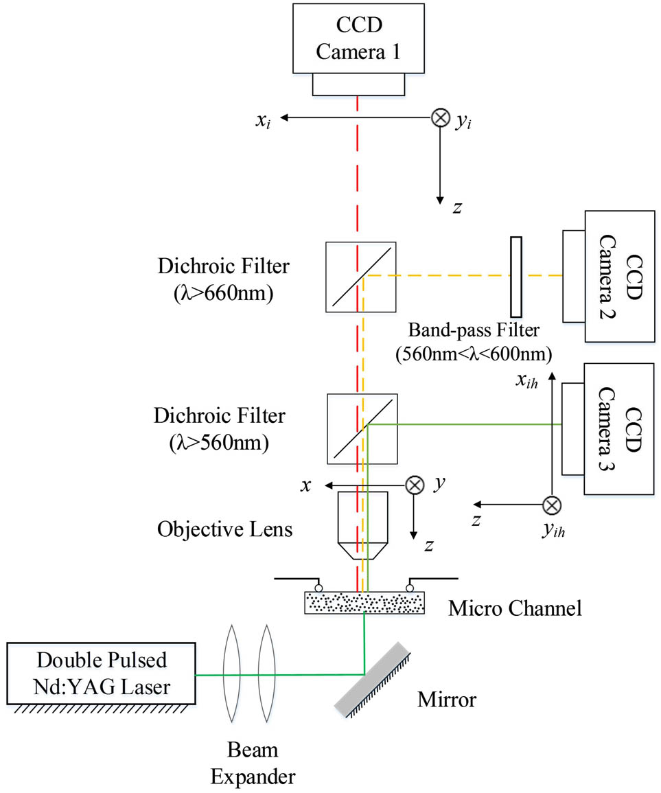
Figure 1 presents a detailed schematic of a typical design of the integrated LIF and micro-DHPTV system. A double pulsed laser $(λ = 532 nm)$ is expanded to a plane wave before illuminating the test section. The fluorescent dyes, temperature-insensitive sulforhodamine 101 (SRh101) and temperature-sensitive rhodamine B (RhB), on the tracer particles are excited. With the help of the dichroic filters and band-pass filter, the fluorescence emitting from SRh101 and RhB is separated and recorded by CCD 1 $(λ > 660 nm)$ and CCD 2 $(560 nm < λ < 600 nm)$ , respectively. At the same time, scattering light $(λ = 532 nm)$ from the particles interferes with the undisturbed incident wave to form a hologram pair that is recorded by CCD 3. Given that the particles are usually semi-transparent polymeric spheres, we do not necessarily use an epi-fluorescent microscope geometry.

Sign up for Chinese Optics Letters TOC. Get the latest issue of Chinese Optics Letters delivered right to you！Sign up now

Figure 1.Integrated two-color LIF and micro-DHPTV system.

In two-color LIF thermometry, the fluorescence intensity of the temperature-sensitive dye is usually dependent on temperature, while the temperature-insensitive dye is used as the reference dye. The intensity ratio of the two fluorescence emissions on a tracer particle is used to determine the temperature and can be directly expressed as^[8] $\frac{I_{RhB}}{I_{SRh 101}} = \frac{I_{in} C_{RhB} ε_{RhB} Q_{RhB}}{I_{in} C_{SRh 101} ε_{SRh 101} Q_{SRh 101}},$ (1)where $I$ represents the fluorescence intensity, $I_{in}$ is the incident light intensity, $C$ is dye concentration, $ε$ is the absorption coefficient, and $Q$ is quantum efficiency. The ratio of the absorption coefficient and incident intensity of the two dyes is invariant. Assuming that the dye concentration on each particle is the same, the fluorescence intensity ratio is solely dependent on $Q_{RhB} / Q_{SRh 101}$ , which is a function of the local temperature. Consequently, tracer particles can be used as local temperature sensors.

As a microscopic imaging system is limited by the depth-of-field (typically 1–10 μm), defocused images of particles should be analyzed. A diffraction-based model^[13] is adopted to describe defocused particle images, based on two hypotheses: (i) fluorescence is regarded as incoherent light; (ii) fluorescence cropped by the filters is in such a narrow band range that the recorded fluorescence light from RhB and SRh101 is simplified as single wavelength emission at 580 and 660 nm, respectively. The image intensity of the fluorescent particle is then given by^[13] $I_{i} (x_{i}, y_{i}) = F^{- 1} {F [{| h (x_{i}, y_{i}) |}^{2}] \cdot F [I_{g} (x_{i}, y_{i})]},$ (2) $I_{g} (x_{i}, y_{i}) = \frac{1}{M^{2}} I_{0} (- \frac{x_{i}}{M}, - \frac{y_{i}}{M}),$ (3)where $I_{i}$ is the image intensity recorded by the CCD camera, $I_{g}$ is the ideal image intensity of the object $I_{0}$ that is derived from the geometrical optics, $M$ is the magnification of the imaging system, and $F$ denotes the Fourier transform. The amplitude impulse response $h$ reads as $h (x_{i}, y_{i}) = F^{- 1} [H (f_{X}, f_{Y})],$ (4) $H (f_{X}, f_{Y}) = P (λ z_{i} f_{X}, λ z_{i} f_{Y}) \exp [j k W (λ z_{i} f_{X}, λ z_{i} f_{Y})],$ (5)where $H$ is the amplitude transfer function, $λ$ is the working wavelength, $z_{i}$ represents the distance of the plane of lens exit from the ideal image plane, and $f_{X}$ and $f_{Y}$ are the corresponding spatial frequency at the point $(x, y)$ of the exit pupil with $x = λ z_{i} f_{X}$ and $y = λ z_{i} f_{Y}$ , respectively. The highest frequency of the image is determined by the numerical aperture (NA) of the lens as well as pixel size of the CCD camera. Term $P$ is a pupil function defined by $P (x, y) = {\begin{matrix} 1 & inside the lens aperture \\ 0 & otherwise \end{matrix} .$ (6)In Eq. (5), $k = 2 π / λ$ and the aberration function $W$ is an effective path-length error that quantitatively describes the wavefront error at the exit pupil compared to a perfect spherical wave. Research has shown that the image of a defocused fluorescent particle is usually dominated by the focusing error and spherical lens aberration^[5] and this approximation is adopted in our model. It is well-known that the primary spherical aberration at $(x, y)$ is proportional to the fourth power of normalized pupil radius^[14]; thus $W$ is written as $W (x, y) = - \frac{1}{2} (\frac{1}{z_{a}} - \frac{1}{z_{i}}) (x^{2} + y^{2}) + Φ \frac{{(x^{2} + y^{2})}^{2}}{r^{4}} .$ (7)where $r$ is the radius of exit pupil. The first term on the right of Eq. (7) denotes focusing error and the second term denotes spherical aberration. Term $z_{a}$ is the distance of the plane of lens exit from the recording plane. Since different lenses have different spherical aberrations, it is unnecessary to determine the spherical aberration of a certain lens and here we identify the coefficient $Φ = 0.5 λ$ to take spherical aberration into consideration^[14].

Figure 2 shows the results of the model and those of a real imaging system. Defocused particle images of 2.9 μm and their intensity distributions are compared. For simulation, the imaging system had a magnification of $20 \times$ , $NA = 0.45$ . The working wavelength was set as 580 nm. For experiments, 2.9 μm RhB fluorescent particles (Duke Scientific) were studied using a Zeiss inverted fluorescent microscope (Axiovert 200). A mercury lamp was used as the light source, in connection with a filter cube. A lens of $20 \times$ , $NA = 0.45$ was used such that the condition was similar to that in the simulation. Images were recorded using a CCD camera (PCO 1400) containing $1392 pixels \times 1040 pixels$ , 6.45 μm/pixel.

Figure 2.Defocused fluorescent particle: (a) experimental images, calibrated magnification of 15.1; (b) simulated images; (c) intensity distribution at $z = - 40 μm$ ; (d) intensity distribution at $z = 30 μm$ . Each image is $106 pixels \times 106 pixels$ , 6.45 μm/pixel at the imaging plane.

The simulated images [Fig. 2(b)] have the same structure with the experimental results [Fig. 2(a)]. The image tends to have a bright outer ring at the $- z$ positions, then the ring disappears and the image becomes a bright center with blurred boundary when moving to the $+ z$ positions. Figures 2(c) and 2(d) present intensity distributions of experimental and simulated images at $z = - 40 μm$ and $z = 30 μm$ , respectively. The curves basically fit well, but the experimental curves have more fluctuations and show lower contrast. This is because the background noises render the image slightly different from an ideal pattern. Particle defects such as nonspherical shape and nonuniform fluorescent dye also lead to slight difference from the ideal defocused pattern. The simulated particle is qualified to describe a real particle nevertheless.

For the purpose of obtaining intensity ratio of two dyes on the same particle, the intensities recorded by CCD 1 and CCD 2 should be mutually normalized. Such a normalization processing is what happens in most multi-camera systems, e.g., a tomographic particle image velocimetry (PIV) system. Meanwhile, a pair of particle holograms are sequentially recorded by CCD 3 to track the particles. Simulated images of 30 tracer particles are presented in Fig. 3. Figures 3(a) and 3(b) are simulated fluorescence images with the previously proposed model and the intensity ratio is used to measure temperature. Figures 3(c) and 3(d) are a corresponding hologram pair that is calculated using the Generalized Lorenz–Mie theory (GLMT)^[15,16].

Figure 3.Simulation images of 30 tracer particles: (a) fluorescence image of RhB; (b) fluorescence image of SRh101; (c) hologram of the first frame; (d) hologram of the second frame.

Defocused particles can be detected with the same method as defocusing micro-PTV^[6] and matched with the help of coordinate system calibration^[7]. The local average intensity around each particle pair was calculated and the intensity ratio was obtained. Particle positions were retrieved from the holograms reconstructed with the convolution approach^[17]. To determine the $z$ position, a wavelet-based autofocusing algorithm was adopted^[18]. Then both the reconstructed particle field and the original holograms were used to track particles with the integrated nearest neighbor and cross correlation pairing methods^[19]. Figure 4 analyzes the position error and the displacement error of the simulated particles. These particles are distributed at different $z$ positions from $- 40$ to 40 μm, thus the recording distances of the holograms vary from 60 to 140 μm. As the $z$ position accuracy is limited by the low NA of a digital holographic system, the $z$ position error is larger than the $x - y$ position error, as shown in Fig. 4(a), which also results in larger $z$ displacement error [Fig. 4(b)]. Relative displacement error in Fig. 4(b) decreases rapidly with respect to the increasing displacement, ensuring the accuracy of velocity measurements. Figure 5 illustrates that intensity ratio with respect to different $z$ positions from $- 40$ to 40 μm nearly remains constant and agrees well with a linear fit. This fit can be used to calibrate the intensity ratio if necessary. Accordingly, the effect of the $z$ position error on the intensity ratio is no more than 1.5%, which leads to the temperature error of less than 1°C. Consequently, the ratiometric fluorescence temperature sensors can work at a wide range of depth positions. Similar results have also been reported with elaborately designed experiments^[10]. In an experimental optical system, dilute suspension of tracer particles should be concerned to suppress background noises. High light sensitivity of the CCD camera (12 bits) is needed to ensure successful detection of defocused particles.

Figure 4.Particle position and displacement errors: (a) position error; (b) displacement error.

Figure 5.Intensity ratio at different $z$ positions.

To evaluate the effectiveness of the combined two-color LIF and micro-DHPTV system, the method was tested in numerical work. An imaginary flow field in the volume of $120 μm (length) \times 120 μm (width) \times 80 μm (depth)$ was designed with all the parameters detailed in Table 1. The flow had a velocity in the $x$ direction that met a parabolic distribution [colored surface in Fig. 6(a)]. The temperature distribution [red line in Fig. 6(b)] was set linear along the $x$ direction. Fluorescent particles with a diameter of 2.9 μm were randomly and uniformly distributed in the test volume with a particle concentration of 30 particles in one image. The holograms simulated with GMLT were reconstructed to retrieve the positions and velocities of the particles. Fluorescence emissions from each particle were used to measure local temperature. To restore the 3D temperature and velocity fields of the flow, superposition of 14 groups of images with 420 tracer particles were used.

Figure 6.Velocity distribution and temperature distribution of the flow field: (a) velocity distribution; (b) temperature distribution.

Item	Description	Parameter
Velocity	ux=u0r02(r02−y2−z2)	u0=0.07 m/sr0=75 μmΔt=100 μs
Temperature	T=T0+axx0	T0=40°Cx0=60 μma=1/3
Dye 1	RhB	Temperature sensitivity 1.5%/°C^[7]
Dye 2	SRh101	Temperature sensitivity 0.17%/°C^[7]

Table 1. Parameters of the Numerical Test

View all Tables

Figure 6 compares the numerical results with the theoretical value of the flow field. Circular markers in Fig. 6(a) represent particle velocity distribution in the $y - z$ cross section, with the height indicating velocity magnitude. The colored surface denotes the theoretical velocity distribution of the flow, with the color proportional to the velocity magnitude. Despite some pairing failures, most particles are accurately tracked and the local velocities reflect the flow field well. Figure 6(b) displays temperature distribution along the $x$ direction. The blue spots are the result of numerical tests, with all spots accumulating to the red line which signifies the theoretical value. Figure 7 shows the superimposed 3D temperature and velocity field from 391 valid particles. Small spheres in the field represent tracer particles with the color proportional to the local temperature; the arrow associated with the particle implies both the direction and magnitude of local velocity. Particles have larger velocity in the center than on the edges, and the temperature increases when particles travel along the $x$ axis.

Figure 7.Visualization of 3D temperature and velocity field.

In conclusion, a method to simultaneously characterize the 3D temperature and velocity field of micro-flow is proposed, based on a combination of two-color LIF and micro-DHPTV. We use a diffraction-based model to describe defocused fluorescent particle images. By comparing the simulated images with experimental images, we find that the model works well. The intensity ratio at different $z$ positions shows little difference, which indicates that defocused LIF particles can be used to measure the temperature. The 3D temperature and velocity of a presupposed micro-flow field in a $120 μm \times 120 μm \times 80 μm$ region is then tested. The numerical results show good overall agreement with the theoretical value.