• Matter and Radiation at Extremes
  • Vol. 6, Issue 2, 026902 (2021)
Qianrui Liu1, Junyi Li2, and Mohan Chen1、a)
Author Affiliations
  • 1CAPT, HEDPS, College of Engineering, Peking University, Beijing 100871, People’s Republic of China
  • 2School of Computer Science and Technology, Harbin Institute of Technology (Shenzhen), Shenzhen, Guangdong 518055, People’s Republic of China
  • show less
    DOI: 10.1063/5.0030123 Cite this Article
    Qianrui Liu, Junyi Li, Mohan Chen. Thermal transport by electrons and ions in warm dense aluminum: A combined density functional theory and deep potential study[J]. Matter and Radiation at Extremes, 2021, 6(2): 026902 Copy Citation Text show less

    Abstract

    We propose an efficient scheme that combines density functional theory (DFT) with deep potentials (DPs), to systematically study convergence issues in the computation of the electronic thermal conductivity of warm dense aluminum (2.7 g/cm3 and temperatures ranging from 0.5 eV to 5.0 eV) with respect to the number of k-points, the number of atoms, the broadening parameter, the exchange-correlation functionals, and the pseudopotentials. Furthermore, we obtain the ionic thermal conductivity using the Green–Kubo method in conjunction with DP molecular dynamics simulations, and we study size effects on the ionic thermal conductivity. This work demonstrates that the proposed method is efficient in evaluating both electronic and ionic thermal conductivities of materials.

    I. INTRODUCTION

    Warm dense matter (WDM) is a state of matter lying between condensed matter and plasma and consisting of strongly coupled ions and partially degenerate electrons. WDM exists in the interiors of giant planets1,2 and in the crusts of white dwarf and neutron stars,3,4 and it can be generated through laboratory experiments with diamond anvil cells,5 gas guns,6,7 and high-power lasers.7,8 WDM also plays an important role in inertial confinement fusion (ICF).9 In these contexts, it is crucial to understand the properties of WDM such as its equation of state and its optical and transport properties. Owing to the lack of experimental data, quantum-mechanics-based simulation methods such as Kohn–Sham density functional theory (KSDFT),10,11 orbital-free density functional theory (OFDFT),12 and path-integral Monte Carlo13–16 have emerged as ideal tools to study WDM.16–20 Thermal conductivity is one of the most important properties of WDM. For example, it has been widely studied in the context of models of planetary interiors.21–23 It is a key parameter governing the growth of hydrodynamic instabilities that arise with various capsule designs for the National Ignition Facility.24 It also plays a key role in simulations of the interactions between lasers and metal targets.25 The thermal conductivity has a significant influence on predictions of ICF implosions in hydrodynamic simulations.26

    The thermal conductivity includes both electronic and ionic contributions. The Kubo–Greenwood (KG) formula27,28 has been widely used in studies of the electronic thermal conductivity κe of liquid metals and WDM.18,26,29–35 Typically, the κe value is an average of results from several atomic configurations, which are selected from first-principles molecular dynamics (FPMD) simulations. However, it is computationally expensive to perform FPMD simulations for large systems, especially for WDM when the temperatures are high.19,33,36,37 Besides, it has been shown that size effects may substantially affect κe.30,33,38 For computations of the ionic thermal conductivity κI, we focus on the Green–Kubo (GK) formula,27,39,40 where κI is expressed in terms of the heat flux autocorrelation function, which requires knowledge of the energy and the virial tensor of each atom from the molecular dynamics trajectory. Typically, this formula is used with empirical force fields,41–43 since traditional DFT methods cannot yield an explicit energy for each atom; note that ab initio GK formulas for evaluation of κI have been proposed in some recent work.44–47 Besides, a long molecular dynamics trajectory may be needed to evaluate κI, which poses another challenge for DFT simulations.

    While current experimental techniques only measure the total thermal conductivity, first-principles methods have become ideal tools to yield electronic and ionic contributions separately. However, only a few studies adopting first-principles methods have examined transport properties by considering both contributions.32,48,49 For some metals, the ionic contribution is not important,48 but this is not the case for all metals, tungsten being one example.49 In addition, first-principles methods are computationally expensive, especially when a large system or a long trajectory is considered. In this regard, there is a need for an efficient and accurate method that can yield both electronic and ionic thermal conductivities of materials. Here, using the KG and GK formulas, we propose a combined DFT and deep potential (DP) method for this purpose, taking warm dense Al as an example. The recently developed DP molecular dynamics (DPMD)50–52 method learns first-principles data via deep neural networks and yields a highly accurate many-body potential to describe the interactions among atoms. Compared with traditional DFT, DPMD has a much higher efficiency while retaining the ab initio accuracy. In addition, linear-scaling DPMD can be parallelized to simulate hundreds of millions of atoms.53,54 The DP method has been applied in a variety of contexts, such as crystallization of silicon,55 high-entropy materials,56 and isotope effects in liquid water,57,58 as well as WDM.59,60

    In this work, we demonstrate that the DP method in conjunction with DFT can be used to obtain both electronic and ionic thermal conductivities of warm dense Al. We use KSDFT, OFDFT, and DPMD to study the electronic and ionic thermal conductivities of warm dense Al at temperatures of 0.5 eV, 1.0 eV, and 5.0 eV with a density of 2.7 g/cm3. The electronic thermal conductivity can be accurately computed via the KG method based on the DPMD trajectories instead of the FPMD trajectories. Importantly, we systematically investigate convergence issues with regard to the number of k-points, the number of atoms, the broadening parameter, the exchange-correlation functionals, and the pseudopotentials, together with their effects on the determination of the electronic thermal conductivity via DPMD simulations. Furthermore, the ionic thermal conductivity can also be obtained via DPMD simulations, and we study convergence for different sizes of systems and different lengths of trajectories.

    The remainder of the paper is organized as follows. In Sec. II, we briefly introduce KSDFT, OFDFT, and DPMD, as well as the setups of the simulations. We also briefly introduce the KG and GK formulas that are used in this work. In Sec. III, we present the electronic thermal conductivities computed using each of the three methods. We then give a thorough discussion of convergence issues as they affect the electronic thermal conductivity. Finally, we present results for the ionic thermal conductivity of warm dense Al. We conclude our work in Sec. IV.

    II. METHOD

    A. Density functional theory

    The ground-state total energy within the formalism of DFT10,11 can be expressed as a functional dependence of the electron density. The Hohenberg–Kohn theorems10 point out that the electron density that minimizes the total energy is the ground-state density, while the energy is the ground-state energy.10 Depending on the way in which the electron kinetic energy is treated, there are two DFT methods, namely, KSDFT11 and OFDFT.12 The electron kinetic energy in KSDFT does not involve the electron density explicitly, but is evaluated from the ground-state wave functions of electrons obtained by self-consistent iterations. On the other hand, in OFDFT, the electron kinetic energy is given approximately as an explicit density functional,61–65 which enables a direct search for the ground-state density and energy. As a result, KSDFT has higher accuracy, but OFDFT is several orders more efficient, especially for large systems. Mermin extended DFT to finite temperatures,66 in an approach that has been widely used to describe electrons in WDM.18,29

    We run 64-atom Born–Oppenheimer molecular dynamics (BOMD) simulations with KSDFT using the Quantum ESPRESSO 5.0.2 package.67 The Perdew–Burke–Ernzerhof (PBE) exchange-correlation (XC) functional68 is used. The projector augmented-wave (PAW) potential69,70 is used, with three valence electrons and a cutoff radius of 1.38 Å. The plane wave cutoff energy is set to 20 Ry for temperatures of 0.5 eV and 1.0 eV and to 30 Ry for 5.0 eV. We only use the gamma k-point. Periodic boundary conditions are adopted. The Andersen thermostat71 is used with the NVT ensemble, and the trajectory length is 10 ps, with a time step of 1.0 fs.

    We also perform 108-atom BOMD simulations with OFDFT, using the PROFESS 3.0 package.72 Both PBE68 and local density approximation (LDA)11 XC functionals are used, together with the Wang–Teter (WT) kinetic energy density functional (KEDF)65 and the Nosé–Hoover thermostat73,74 in the NVT ensemble. We run OFDFT simulations for 10 ps, with a time step of 0.25 fs, and we set the energy cutoff to 900 eV. Periodic boundary conditions are adopted.

    B. Deep potential molecular dynamics

    The DP method50–52 learns the dependence of the total energy on the coordinates of the atoms in a system and constructs a deep neural network (DNN) model that predicts the potential energy and force of each atom. In the training process, the total potential energy Etot is decomposed into the energies of the different atoms:Etot=iEi,where Ei is the potential energy of atom i. In general, through the DNN, for each atom i, a mapping is established between Ei and the atomic coordinates of its neighboring atoms within a cutoff radius rc. Specifically, the DNN model consists of an embedding network and a fitting network.50 The embedding network imposes constraints on the atoms, such that the atomic coordinates obey symmetries under translation, rotation, and permutation. On the other hand, the fitting network maps the atomic coordinates from the embedding network to Ei. Next, the training data are prepared as the total energy and the forces acting on atoms are extracted from the FPMD trajectories. Finally, the parameters of the DNN model are optimized by minimizing a loss function. The resulting DNN-based model can be used to simulate a large system with an efficiency comparable to that when empirical force fields are used.

    In this work, we adopt DNN-based models trained from either KSDFT or OFDFT trajectories with the DeePMD-kit package.51 With the purpose of studying size effects on electronic thermal conductivity, a series of cubic cells consisting of 16, 32, 64, 108, 216, and 256 atoms are simulated for 10 ps with a time step of 0.25 fs. In addition, we run systems of 16, 32, 64, 108, 256, 1024, 5488, 8192, 10 648, 16 384, 32 000, and 65 536 atoms to investigate the convergence of the ionic thermal conductivity. The length of these trajectories is 500 ps, with a time step of 0.25 fs. We employ the Nosé–Hoover thermostat73,74 in the NVT ensemble. Periodic boundary conditions are adopted. All of the DPMD simulations are performed using the modified LAMMPS package.75

    C. Kubo–Greenwood formula

    The electronic thermal conductivity κe is calculated from the Onsager coefficients Lmn asκe=1e2TL22L122L11,where T is the temperature and e is the electron charge. The Lmn are obtained as the zero-frequency limits of the frequency-dependent Onsager coefficients Lmn(ω):Lmn=limω0Lmn(ω).We follow the approach to the KG formula adopted by Holst et al.,76 according to which the Lmn(ω) are given byLmn(ω)=(1)m+n2πe223me2ωΩ×ijαkW(k)ϵik+ϵjk2μm+n2|Ψik|α|Ψjk|2×[f(ϵik)f(ϵjk)]δ(ϵjkϵikω),where me is the electron mass, Ω is the cell volume, W(k) is the weight of k-points in the Brillouin zone, μ is the chemical potential, Ψik is the wave function of the ith band with eigenvalue ϵik, and f is the Fermi–Dirac function. We use the chemical potential μ instead of the enthalpy per atom, which does not affect the results for the electronic thermal conductivity in one-component systems.76 Note that here we use the momentum operator in Eq. (4) instead of the velocity operator, and this introduces additional approximations due to the use of nonlocal pseudopotentials.18,34,77–79 However, the nonlocal errors have been demonstrated to be about 3.3% for liquid Al,78 and this is considered to be sufficiently small for the purposes of this work. In the future work, we will include the additional term caused by nonlocal pseudopotentials. We also define the frequency-dependent electronic thermal conductivity asκe(ω)=1e2TL22(ω)L122(ω)L11(ω).In practical applications of the KG method, the delta function in Eq. (4) needs to be broadened. We adopt a Gaussian function,29 and the delta function then takes the formδ(E)=limΔE012πΔEeE2/2ΔE2.Here, ΔE controls the full width at half maximum (FWHM, denoted by σ) of the Gaussian function through the relation σ ≈ 2.3548ΔE.

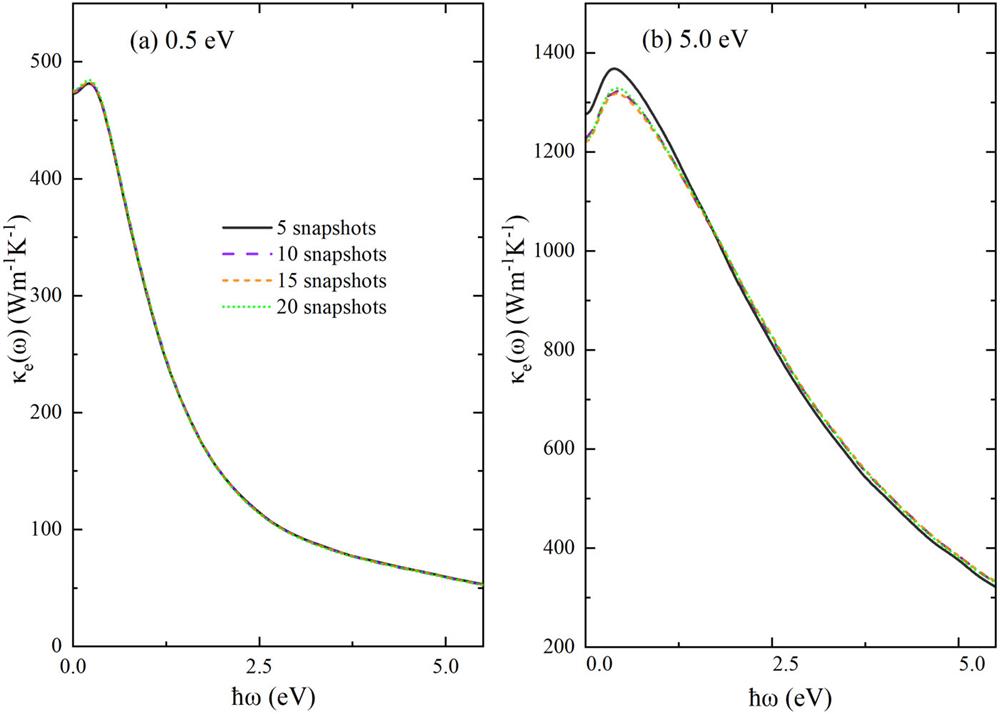
    The KG method needs eigenvalues and wave functions computed from DFT solutions of given atomic configurations. In practice, we select 5–20 atomic configurations from the last 2 ps MD trajectories, with a time interval of 0.1 ps. We use both PBE and LDA XC functionals and the associated norm-conserving (NC) pseudopotentials to examine the influences of XC functionals and pseudopotentials on the resulting electronic thermal conductivity. We adopt two NC pseudopotentials for Al, which are referred to here as PP1 and PP2. The PP1 pseudopotential is generated with the optimized norm-conserving Vanderbilt pseudopotential method via the ONCVPSP package.80,81 We use 11 valence electrons and a cutoff radius of 0.50 Å. Our calculations of κe in a 64-atom cell involve 1770, 2100, and 5625 bands at temperatures 0.5 eV, 1.0 eV, and 5.0 eV, respectively. The PP2 pseudopotential is generated through the PSlibrary package.82 We use the Troullier–Martins method,83 and the cutoff radius is set to 1.38 Å. We choose three valence electrons for each atom. We select 720, 1100, and 4800 bands for calculations of κe at temperatures 0.5 eV, 1.0 eV, and 5.0 eV, respectively. The plane wave cutoff energies of both pseudopotentials are set to 50 Ry. Generally, the PP1 pseudopotential is used in most cases, with the PP2 pseudopotential only being used to compare the effects of different pseudopotentials on κe. Figure 1 shows the computed averaged κe(ω) with respect to different numbers of atomic configurations from 108-atom DPMD trajectories at 0.5 eV and 5.0 eV. The DP model is trained based on the 108-atom OFDFT trajectories using the PBE XC functional. We can see that 20 atomic configurations are enough to converge κe(ω). Additionally, κe(ω) converges more easily at the relatively low temperature of 0.5 eV. Therefore, we choose 20 atomic configurations for cells with 108 atoms or less at all the three temperatures. For systems with more than 108 atoms, we respectively select 5 and 10 atomic configurations for temperatures smaller than 5.0 eV and equal to 5.0 eV, unless otherwise specified.

    Convergence of frequency-dependent electronic thermal conductivity κe(ω) of Al with respect to the number of atomic configurations (snapshots) selected from DPMD trajectories. The temperature is set to (a) 0.5 eV and (b) 5.0 eV. The number of snapshots used together with the KG formula (the broadening parameter is set to 0.4 eV) is shown by different line styles. The DP model is trained from the OFDFT trajectories using the PBE XC functional. The simulation cell contains 108 atoms.

    Figure 1.Convergence of frequency-dependent electronic thermal conductivity κe(ω) of Al with respect to the number of atomic configurations (snapshots) selected from DPMD trajectories. The temperature is set to (a) 0.5 eV and (b) 5.0 eV. The number of snapshots used together with the KG formula (the broadening parameter is set to 0.4 eV) is shown by different line styles. The DP model is trained from the OFDFT trajectories using the PBE XC functional. The simulation cell contains 108 atoms.

    D. Green–Kubo formula

    In the DPMD method, the total potential energy of the system is decomposed onto each atom. In this regard, the ionic thermal conductivity can be calculated through the GK method40 with the formulaκI=13ΩkBT20+Jq(t)Jq(0)dt,where Ω is the cell volume, T is the temperature, kB is the Boltzmann constant, 〈⋯〉 is the ensemble average, and t is time. Jq in Eq. (7) is the heat current of a one-component system in the center-of-mass frame and takes the formJq=i=1Nεivi12i=1NjiN(viFij)rij.Here, vi is the velocity of the ith atom, and ɛi is the energy of the ith atom including ionic kinetic energy and potential energy, where the potential energy is directly obtained by the DNN. Fij is the force acting on the ith atom due to the presence of the jth atom, with rij defined as rirj. It is worth mentioning that Eq. (8) is valid for two-body potentials but yields an error of about 20% in Jq when a many-body potential (e.g., the deep potential) is adopted.84 Importantly, as will be shown below, the ionic thermal conductivity of warm dense Al is at least two orders of magnitudes smaller than the electronic thermal conductivity. Therefore, we still consider Eq. (8) as a valid but approximate formula to yield the ionic thermal conductivity of warm dense Al with DPMD. Additionally, we recommend the use of a more complete formula for those systems whose ionic thermal conductivity is an important part of the total thermal conductivity.

    Equation (7) can also be written asκI=0+CJ(t)dt,from which the autocorrelation function of the heat current is defined asCJ(t)=13ΩkBT2Jq(t)Jq(0).

    III. RESULTS

    A. Accuracy of DP models

    We first perform FPMD simulations of Al based on KSDFT and OFDFT at temperatures of 0.5 eV, 1.0 eV, and 5.0 eV. The PBE XC functional is used, and the FPMD trajectory length is 10 ps. The cell contains 64 Al atoms. Two DP models, named DP-KS and DP-OF, are trained, based on the KSDFT and OFDFT trajectories, respectively. Note that the accuracy of the DP models in describing warm dense Al at the three temperatures has been demonstrated in our previous work,59 where we showed that DPMD has excellent accuracy in reproducing structural and dynamical properties, including radial distribution functions and static and dynamic structure factors.

    Here, we first focus on the frequency-dependent Onsager coefficients Lmn(ω). Figure 2 shows the L11(ω), L12(ω), and L22(ω) computed via different methods at 0.5 eV; L21(ω) is not shown, since L21(ω) = L12(ω), as derived from Eq. (4). We can see that for L11(ω) and L22(ω) all four methods yield very similar results, but for L12(ω) there are deviations at low frequencies. The main reason for this is the greater sensitivity of L12(ω) to the number of ionic configurations, and 20 snapshots are not enough to provide good convergence. We also run a test with 40 snapshots, and this improves the results, as can be seen in Fig. 2(d). However, the resulting electronic thermal conductivity depends mainly on L22(ω) at the temperatures considered in this work, and so the small deviations in L12(ω) do not affect the computed κe(ω), as will be shown next.

    Frequency-dependent Onsager kinetic coefficients (a) L11, (b) L12, and (c) L22 of Al at a temperature of 0.5 eV as computed using the KS, OF, DP-KS, and DP-OF methods. DP-KS and DP-OF refer to the DP models trained from OFDFT and KSDFT molecular dynamics trajectories, respectively. The broadening parameter used in the KG method is set to 0.4 eV. The simulation cell contains 64 Al atoms. (d) shows the improvement in the results for L12 obtained by using 40 rather than 20 snapshots.

    Figure 2.Frequency-dependent Onsager kinetic coefficients (a) L11, (b) L12, and (c) L22 of Al at a temperature of 0.5 eV as computed using the KS, OF, DP-KS, and DP-OF methods. DP-KS and DP-OF refer to the DP models trained from OFDFT and KSDFT molecular dynamics trajectories, respectively. The broadening parameter used in the KG method is set to 0.4 eV. The simulation cell contains 64 Al atoms. (d) shows the improvement in the results for L12 obtained by using 40 rather than 20 snapshots.

    The results for the frequency-dependent electronic thermal conductivity κe(ω) computed using the four different methods are illustrated in Fig. 3. We can see that the OFDFT results agree well with the KSDFT ones, suggesting that OFDFT has the same accuracy as KSDFT in yielding atomic configurations for subsequent computations of κe(ω) via the KG method, even though some approximations are made with regard to the electron kinetic energy65 and the local pseudopotential85 within the framework of OFDFT. Impressively, the DP models trained from FPMD trajectories yield almost identical κe(ω) when compared with the DFT results, which proves that the DP models can yield highly accurate atomic configurations for subsequent calculations of κe(ω). In conclusion, the input atomic configurations for the calculation of κe(ω) can be generated by efficient DPMD models without loss of accuracy, which is beneficial for simulating a large number of atoms to mitigate size effects. Although the preparation of the training data in the DPMD model requires additional computational resources, we find that running FPMD with a cell consisting of 64 atoms is sufficient to generate reliable DPMD models. Therefore, additional computational costs are saved once larger numbers of atoms are adopted in the linear-scaling DPMD method.59

    Frequency-dependent electronic thermal conductivity κe(ω) as computed using the KG method (the broadening parameter is set to 0.4 eV) with snapshots from KS, OF, DP-KS, and DP-OF molecular dynamics trajectories. The temperatures are (a) 0.5 eV, (b) 1.0 eV, and (c) 5.0 eV. DP-KS and DP-OF refer to the DP models trained from OFDFT and KSDFT molecular dynamics trajectories, respectively. The cell contains 64 Al atoms.

    Figure 3.Frequency-dependent electronic thermal conductivity κe(ω) as computed using the KG method (the broadening parameter is set to 0.4 eV) with snapshots from KS, OF, DP-KS, and DP-OF molecular dynamics trajectories. The temperatures are (a) 0.5 eV, (b) 1.0 eV, and (c) 5.0 eV. DP-KS and DP-OF refer to the DP models trained from OFDFT and KSDFT molecular dynamics trajectories, respectively. The cell contains 64 Al atoms.

    B. Convergence of electronic thermal conductivity

    Previous work30,33,38 has shown that the electronic thermal conductivity κe depends strongly on both the number of k-points and the number of atoms. Additionally, the broadening parameter should be chosen appropriately to yield a meaningful κe. Here, we systematically investigate these issues by adopting the DPMD model to generate atomic configurations for subsequent calculations of κe. The DPMD model is trained from OFDFT-based MD trajectory with the PBE XC functional. By utilizing the snapshots from the DPMD trajectory, we obtain κe by using the KG formula. Furthermore, we study the effects of different XC functionals and pseudopotentials in affecting κe.

    1. Number of k-points

    We first investigate the convergence of κe(ω) with respect to different numbers of k-points. Figure 4 illustrates an example of warm dense Al in a 64-atom cell at a temperature of 1.0 eV. The k-point meshes are chosen to be 1 × 1 × 1, 2 × 2 × 2, 3 × 3 × 3, and 4 × 4 × 4 in the calculations of κe(ω). The results show that κe(ω) converges when 3 × 3 × 3 k-points are used. In fact, the number of k-points required for convergence of κe(ω) varies with different numbers of atoms and at different temperatures. Table I lists the sizes of k-points that are needed to converge κe(ω) with numbers of atoms ranging from 16 to 256 at temperatures of 0.5 eV, 1.0 eV, and 5.0 eV. We find that the number of k-points required exhibits a trend to decrease at higher temperatures. For instance, the numbers of k-point samplings required for a 32-atom cell at temperatures of 0.5 eV, 1.0 eV, and 5.0 eV are 6 × 6 × 6, 5 × 5 × 5, and 3 × 3 × 3, respectively. This can be understood from the fact that the Fermi–Dirac distribution of electrons around the Fermi energy becomes sharper at low temperatures. Therefore, a dense mesh of k-points is needed to represent the detailed structures around the Fermi surface at low temperatures.

    Convergence of frequency-dependent electronic thermal conductivity κe(ω) of Al with respect to the number of k-points. The temperature is set to 1.0 eV. The k-point samplings utilized with the KG method (the broadening parameter is set to 0.4 eV) are chosen from 1 × 1 × 1 to 4 × 4 × 4. The DP model is trained from the OFDFT trajectories using the PBE XC functional. The cell consists of 64 atoms.

    Figure 4.Convergence of frequency-dependent electronic thermal conductivity κe(ω) of Al with respect to the number of k-points. The temperature is set to 1.0 eV. The k-point samplings utilized with the KG method (the broadening parameter is set to 0.4 eV) are chosen from 1 × 1 × 1 to 4 × 4 × 4. The DP model is trained from the OFDFT trajectories using the PBE XC functional. The cell consists of 64 atoms.

    N0.5 eV1.0 eV5.0 eV
    168 × 8 × 87 × 7 × 73 × 3 × 3
    326 × 6 × 65 × 5 × 53 × 3 × 3
    643 × 3 × 33 × 3 × 31 × 1 × 1
    1082 × 2 × 22 × 2 × 21 × 1 × 1
    2162 × 2 × 22 × 2 × 21 × 1 × 1
    2562 × 2 × 22 × 2 × 21 × 1 × 1
    4322 × 2 × 2N/AN/A

    Table 1. Sizes of k-points adopted in KSDFT calculations to converge the electronic thermal conductivity of Al with different numbers N of atoms in the simulation cell at temperatures of 0.5 eV, 1.0 eV, and 5.0 eV.

    2. Number of atoms

    The value of κe(ω) converges not only for a sufficient number of k-points but also for a sufficient number of atoms in the simulation cell. To demonstrate this, we plot κe(ω) with respect to different numbers of atoms in Fig. 5. For each size of cell, the number of k-points is chosen large enough to converge κe(ω), as listed in Table I. We find the following. First, for temperatures of 0.5 eV, 1.0 eV, and 5.0 eV, we find that a 256-atom system is large enough to converge κe(ω). Second, in most cases, κe(ω) does not monotonically decrease but has a peak at low frequencies ranging from 0.3 eV to 0.6 eV. This peak moves toward ω = 0 when a larger number of atoms is used, and almost disappears in large cells such as the 432-atom cell at 0.5 eV. Similar to what was found in previous work,38 this phenomenon is caused by size effects. Third, κe(ω) converges more rapidly with respect to the number of atoms at high temperatures, suggesting that size effects are less significant at higher temperatures. For example, the values of κe for the 16- and 64-atom systems at 0.5 eV are 59.7% (195.5 W m−1 K−1) and 15.6% (409.3 W m−1 K−1) lower than the value for the 256-atom system (485.1 W m−1 K−1). Meanwhile, the values of κe for the 16- and 64-atom systems at 5.0 eV are only 47.7% (669.7 W m−1 K−1) and 7.5% (1182.2 W m−1 K−1) lower than the value for a 256-atom system (1281.7 W m−1 K−1).

    Convergence of the electronic thermal conductivity κe(ω) with respect to the number of atoms (from 16 to 432) in the simulation cell. The temperature is set to (a) 0.5 eV, (b) 1.0 eV, and (c) 5.0 eV. (d)–(f) are magnified views of the peaks in (a)–(c), respectively. For the temperature of 0.5 eV, two 432-atom snapshots with 2 × 2 × 2 k-points are chosen to test the convergence of κe(ω). The DP model is trained from the OFDFT trajectories using the PBE XC functional. The broadening parameter is set to 0.4 eV.

    Figure 5.Convergence of the electronic thermal conductivity κe(ω) with respect to the number of atoms (from 16 to 432) in the simulation cell. The temperature is set to (a) 0.5 eV, (b) 1.0 eV, and (c) 5.0 eV. (d)–(f) are magnified views of the peaks in (a)–(c), respectively. For the temperature of 0.5 eV, two 432-atom snapshots with 2 × 2 × 2 k-points are chosen to test the convergence of κe(ω). The DP model is trained from the OFDFT trajectories using the PBE XC functional. The broadening parameter is set to 0.4 eV.

    We perform a further analysis to elucidate the origin of the size effects in computations of κe(ω). As Eq. (4) shows, for a given energy interval ϵikϵjk with electronic states i and j at a specific k point, κe(ω) should converge provided there are a sufficient number of electronic eigenstates. However, it can be seen from Fig. 5 that the computed κe(ω) becomes substantially larger at low frequencies as the number of atoms in the simulation cell increases. These results imply that even when there are enough k-points for convergence to be reached, if only a small number of atoms is used, then the small energy intervals obtained from the finite-size DFT calculations do not provide sufficient information to allow evaluation of κe(ω).

    To clarify this issue, we define an energy interval distribution function (EIDF) asg(E)=1Npi>j,kW(k)δ(ϵikϵjkE),where W(k) represents the weights of the k-points used in the DFT calculations, ϵik and ϵjk are the eigenvalues, and Np is a normalization factor. We choose warm dense Al systems at temperatures of 0.5 eV and 5.0 eV, with the selected energy intervals computed from the bands occupied by 3s and 3p electrons, which can be identified from the density of states (DOS), as illustrated in Fig. 6. The energy intervals satisfy the condition that E < 1.0 eV. In addition, we consider the bands within 6.0 eV and 50.5 eV above the chemical potential μ for temperatures of 0.5 eV and 5 eV, respectively. The results for g(E) with respect to different numbers of atoms ranging from 16 to 432 are illustrated in Fig. 7. The EIDF g(E) becomes larger for small E as the number of atoms increases, and it converges when the number of atoms reaches 256 for both temperatures 0.5 eV and 5.0 eV. The increase in g(E) at small E implies that more energy eigenvalues with values close to one another appear in a larger cell with more atoms. In other words, because of the finite number of atoms used in the simulation cell, the energy levels are discretized to some extent, resulting in a lack of energy intervals, especially for those small values. In particular, these small energy intervals are of considerable importance in the evaluation of κe(ω) when ω → 0, as shown in Eq. (4).

    Density of states of a 256-atom cell at temperatures of (a) 0.5 eV and (b) 5.0 eV. The Fermi–Dirac function at the same temperature is plotted as a black solid line. The DP-OF model refers to the DP model trained from OFDFT molecular dynamics trajectories.

    Figure 6.Density of states of a 256-atom cell at temperatures of (a) 0.5 eV and (b) 5.0 eV. The Fermi–Dirac function at the same temperature is plotted as a black solid line. The DP-OF model refers to the DP model trained from OFDFT molecular dynamics trajectories.

    Energy interval distribution function of different cells at (a) 0.5 eV and (b) 5.0 eV. Bands within 6.0 eV and 50.5 eV above the chemical potential μ are considered for temperatures of 0.5 eV and 5 eV, respectively. Different line styles correspond to different numbers of atoms (from 16 to 432) in the simulation cell. The DP model is trained from the OFDFT trajectories using the PBE XC functional.

    Figure 7.Energy interval distribution function of different cells at (a) 0.5 eV and (b) 5.0 eV. Bands within 6.0 eV and 50.5 eV above the chemical potential μ are considered for temperatures of 0.5 eV and 5 eV, respectively. Different line styles correspond to different numbers of atoms (from 16 to 432) in the simulation cell. The DP model is trained from the OFDFT trajectories using the PBE XC functional.

    3. Broadening parameter

    The FWHM broadening parameter σ that appears in the δ(E) function in Eq. (6) substantially affects the resulting electronic thermal conductivity κe(ω) when ω → 0. We therefore investigate the influence of the choice of σ on the computed κe(ω) by analyzing the EIDF g(E). Taking Al at 0.5 eV as an example, we plot in Fig. 8 both g(E) and κe(ω) of a 256-atom cell, which is large enough to converge g(E) or κe(ω), as demonstrated above. When the broadening effect is small (σ = 0.01 eV), g(E) and κe(ω) decrease dramatically below 0.2 eV, which is a consequence of the discrete band energies. Thus, a suitable σ needs to be chosen to compensate for the discrete band energies. For instance, the value of g(E) at E = 0 increases from 0.22 eV−1 (σ = 0.01 eV) to 0.99 eV−1 (σ = 0.4 eV). However, g(E) becomes saturated if too large a σ is applied, resulting in overcorrection of κe(ω) such that the curve at frequencies lower than 0.6 eV decreases. Therefore, to compensate for the discrete band energies while avoiding overcorrection, we choose σ to be 0.4 eV for warm dense Al at all of the temperatures considered in this work. It is worth mentioning that a majority of studies, including this one, treat the broadening parameter as an adjustable variable to yield a better characterized curve of frequency-dependent thermal conductivity.18,29–31,33,34,38 Although some physical criteria have been proposed,86 no definite conclusions have yet been drawn regarding the choice of the adjustable variable. In this work, we choose the adjustable parameter in terms of sufficiently small energy intervals, which are possible when a sufficiently large supercell is used in the DFT calculations. κe at zero frequency is obtained by linear extrapolation and is illustrated in Fig. 9.

    (a) Energy interval distribution function and (b) electronic thermal conductivity of a 256-atom cell at 0.5 eV. The snapshots are from DPMD simulations. The DPMD model is trained from OFDFT trajectories with the PBE XC functional. Different line styles represent different values of the broadening parameter σ.

    Figure 8.(a) Energy interval distribution function and (b) electronic thermal conductivity of a 256-atom cell at 0.5 eV. The snapshots are from DPMD simulations. The DPMD model is trained from OFDFT trajectories with the PBE XC functional. Different line styles represent different values of the broadening parameter σ.

    Electronic thermal conductivities κe of warm dense Al. DP-KS and DP-OF refer to the DPMD models trained from KSDFT and OFDFT, respectively. Atomic configurations are generated from the DP-KS and DP-OF models. The broadening parameter is set to 0.4 eV. Note that nonlocal corrections have been neglected in this study. Results from Knyazev and Levashov,31 Vlcěk et al.,34 and Witte et al.,87 as well as experimental results from McKelvey et al.,88 are shown for comparison.

    Figure 9.Electronic thermal conductivities κe of warm dense Al. DP-KS and DP-OF refer to the DPMD models trained from KSDFT and OFDFT, respectively. Atomic configurations are generated from the DP-KS and DP-OF models. The broadening parameter is set to 0.4 eV. Note that nonlocal corrections have been neglected in this study. Results from Knyazev and Levashov,31 Vlcěk et al.,34 and Witte et al.,87 as well as experimental results from McKelvey et al.,88 are shown for comparison.

    4. Exchange-correlation functionals

    We study the influences of the LDA and PBE XC functionals on the computed κe(ω) by first validating the atomic configurations generated by FPMD simulations. Specifically, atomic configurations are chosen from two 256-atom DPMD trajectories, which are generated by two DP models trained from OFDFT with the LDA and PBE XC functionals. We then adopt the KG method using the PP1 pseudopotentials generated with the same XC functional and obtain κe at temperatures of 0.5 eV, 1.0 eV, and 5.0 eV. As shown in Fig. 9 and listed in Table II, the κe values obtained from the PBE XC functional are 485.1 W m−1 K−1, 764.1 W m−1 K−1, and 1281.7 W m−1 K−1 at temperatures of 0.5 eV, 1.0 eV, and 5.0 eV, respectively, while the κe values from the LDA XC functional are 1.6% lower (477.3 W m−1 K−1), 1.3% higher (773.8 W m−1 K−1), and 2.8% lower (1246.4 W m−1 K−1) than those from the PBE XC functional at 0.5 eV, 1.0 eV, and 5.0 eV, respectively. Therefore, we conclude that the LDA XC functional yields almost the same κe values as the PBE XC functional. Note that in a recent work87 that adopted the HSE XC functional, there were some differences in the electronic thermal and electrical conductivities of warm dense Al compared with those obtained from the PBE XC functional.

    T (eV)κe(PP1)κe(PP2)κI
    0.5485.1486.61.422 ± 0.034
    DP-OF (PBE)1.0764.1772.31.469 ± 0.086
    5.01281.71604.62.091 ± 0.031
    0.5477.3475.61.394 ± 0.047
    DP-OF (LDA)1.0773.8779.01.318 ± 0.032
    5.01246.41568.52.141 ± 0.051
    0.5466.51.419 ± 0.038
    DP-KS (PBE)1.0771.01.393 ± 0.066
    5.01305.82.075 ± 0.066

    Table 2. Electronic thermal conductivity κe and ionic thermal conductivity κI (both in units of W m−1 K−1) at temperatures T of 0.5 eV, 1.0 eV, and 5.0 eV. The results are computed from the DP-KS and DP-OF molecular dynamics trajectories. DP-KS and DP-OF refer to the DP models trained from KSDFT and OFDFT molecular dynamics trajectories, respectively.

    5. Pseudopotentials

    We investigate how norm-conserving pseudopotentials affect the computed electronic thermal conductivity κe. First of all, Fig. 6 shows the DOS of two types of pseudopotentials (PP1 and PP2) at temperatures of 0.5 eV and 5.0 eV, and we can see that the two pseudopotentials yield similar DOS of 3s3p electrons. Next, Fig. 9 illustrates the computed κe from two types of pseudopotentials and the computed data from Knyazev and Levashov,31 Vlcěk et al.,34 and Witte et al.,87 as well as the experimental data from McKelvey et al.88 The values of κe from the two types of pseudopotentials are also listed in Table II.

    We find the following. First, the DP-OF results agree reasonably well with the DP-KS ones, as has previously been shown in Fig. 3. For example, DP-KS with the PP1 pseudopotential and the PBE XC functional yields κe = 466.5 W m−1 K−1 at 0.5 eV, which is 3.8% lower than that from DP-OF (485.1 W m−1 K−1) at the same temperature, and the relative difference decreases to 1.9% at 5.0 eV. These results indicate that the OFDFT is appropriate for study of the electronic thermal conductivity of warm dense Al in the temperature range from 0.5 eV to 5.0 eV. Second, our calculations with the PP1 and PP2 pseudopotentials yield similar κe values of around 480 W m−1 K−1 and 770 W m−1 K−1 at temperatures of 0.5 eV and 1.0 eV, respectively. The results are consistent with those of Knyazev and Levashov, Vlcěk et al., and Witte et al. However, the κe values from the two pseudopotentials at a temperature of 5.0 eV deviate. For instance, the result from DP-OF (PBE) with the PP2 pseudopotential is 1604.6 W m−1 K−1, while the result with the PP1 pseudopotential is only 1281.7 W m−1 K−1, which is 20.1% lower than the former. The κe values from PP1 are close to those from Witte et al., while the values from PP2 are consistent with Knyazev and Levashov’s data. Note that Witte et al. used a PAW potential with 11 valence electrons and the PBE XC functional, whereas Knyazev and Levashov adopted an ultrasoft pseudopotential with three valence electrons and the LDA XC functional. It is also worth mentioning that Witte et al. used a 64-atom cell, whereas Knyazev and Levashov used a 256-atom cell, and so, according to our analysis, size effects may be present in the former work. In general, both values of electronic thermal conductivity lie within the range of the experimental data obtained by McKelvey et al. Even so, our results demonstrate that different pseudopotentials may substantially affect the results for κe at high temperatures. One possible reason for the deviation of κe at 5.0 eV is the number of electrons included in the pseudopotentials. However, it is also possible that the deviation comes from the fact that the nonlocal potential correction77,78 in Eq. (4) is ignored. Therefore, nonlocal corrections must be considered when calculating the conductivity via the KG formula, and these will be the subject of our future work.

    C. Ionic thermal conductivity

    The ionic thermal conductivity of warm dense Al can be evaluated using the GK formula, since the atomic energies are available in the DPMD method. However, the computed ionic thermal conductivity may be affected by trajectory length and system size. We therefore study the convergence of the ionic thermal conductivity with respect to different lengths of trajectories and system sizes. We first test the convergence of the autocorrelation function CJ(t) in Eq. (10) with respect to different lengths of trajectories, and the results are shown in Fig. 10. A 10 648-atom Al system is considered, with four different lengths of trajectories, namely, 25 ps, 125 ps, 250 ps, and 500 ps, and the DPMD model is trained from OFDFT with the PBE XC functional at a temperature of 0.5 eV. As shown in Fig. 10, the CJ(t) curves abruptly decay within the first 0.1 ps and oscillate with respect to time t. We can see that the oscillations are strongly affected by the length of simulation time. For example, the CJ(t) curve obtained from the 25 ps trajectory exhibits substantially larger oscillations than the curves obtained from the other three trajectories, while the best convergence is achieved with the 250 ps trajectory. These results suggest that to obtain a converged CJ(t) for warm dense Al, a few hundreds of picoseconds are required, even for a system with more than 104 atoms, which is beyond the capability of FPMD simulations but can be realized by DPMD simulations.

    Autocorrelation function of heat current CJ(t) evaluated from different lengths of DPMD trajectories, namely, 25 ps, 125 ps, 250 ps, and 500 ps. The number of Al atoms in the cell is 10 684 and the temperature T = 0.5 eV. The DPMD model is trained from OFDFT with the PBE XC functional.

    Figure 10.Autocorrelation function of heat current CJ(t) evaluated from different lengths of DPMD trajectories, namely, 25 ps, 125 ps, 250 ps, and 500 ps. The number of Al atoms in the cell is 10 684 and the temperature T = 0.5 eV. The DPMD model is trained from OFDFT with the PBE XC functional.

    Next, to examine size effects on the ionic thermal conductivity, we run simulations for 500 ps for 12 different system sizes, with the number of atoms per cell ranging from 16 to 65 536. The results are shown in Fig. 11. Since CJ(t) cannot strictly reach zero, the correlation time t is truncated in the integral of CJ(t) in Eq. (9). In practice, we choose multiple truncations of t ranging from 0.5 ps to 1.5 ps and compute the error bars with the maximum and minimum integral values, which are also shown in Fig. 11. We find that the ionic thermal conductivity increases with increasing system size in the range from 16 to 1024 atoms per cell at all three temperatures considered for warm dense Al. With further increase in system size, the ionic thermal conductivity begins to oscillate until the largest system size is reached (65 536 atoms). We can conclude that at least a 1024-atom system should be adopted and that better convergence of ionic thermal conductivity can be achieved if a larger system is used. A 65 536-atom cell is adopted to compute the ionic thermal conductivity, and the results are shown in Table II. The ionic thermal conductivity of warm dense Al is around 1 W m−1 K−1–2 W m−1 K−1, which is more than two orders of magnitudes smaller than the electronic thermal conductivity. Additionally, it should be noted that the PBE and LDA XC functionals yield similar values for the ionic thermal conductivity.

    Computed ionic thermal conductivity of warm dense Al at (a) 0.5 eV, (b) 1.0 eV, and (c) 5.0 eV for 12 different system sizes. The numbers of atoms per cell in these systems are N = 16, 32, 64, 108, 256, 1024, 5488, 8192, 10 648, 16 384, 32 000, and 65 536. The results are obtained through DPMD trained from OFDFT with the PBE XC functional.

    Figure 11.Computed ionic thermal conductivity of warm dense Al at (a) 0.5 eV, (b) 1.0 eV, and (c) 5.0 eV for 12 different system sizes. The numbers of atoms per cell in these systems are N = 16, 32, 64, 108, 256, 1024, 5488, 8192, 10 648, 16 384, 32 000, and 65 536. The results are obtained through DPMD trained from OFDFT with the PBE XC functional.

    IV. CONCLUSIONS

    We have proposed a method that combines DPMD and DFT to calculate both electronic and ionic thermal conductivities of materials, with the DP models being trained from DFT-based MD trajectories. The resulting DP models accurately reproduce the properties predicted by DFT. In addition, they can be utilized to efficiently simulate a large cell consisting of hundreds of atoms, which largely mitigates the size effects caused by periodic boundary conditions. By taking the atomic configurations from DPMD trajectories, we can use the eigenvalues and eigenstates of a given system obtained from DFT solutions and employ the KG formula to compute the electronic thermal conductivity. In addition, the DP models yield atomic energies, which are not available in the traditional DFT method. By using the atomic energies to evaluate the ionic thermal conductivity, both electronic and ionic contributions to the thermal conductivity can be obtained for a given material.

    We took warm dense Al as an example and thoroughly studied its thermal conductivity. Expensive FPMD simulations of large systems can be replaced by DPMD simulations with much smaller computational resources. We first computed the temperature-dependent electronic thermal conductivities of warm dense Al from 0.5 eV to 5.0 eV at a density of 2.7 g/cm3 with snapshots from OFDFT, KSDFT, and DPMD, and the three methods yielded almost the same results, demonstrating that the DPMD method has similar accuracy to FPMD simulations. We then systematically investigated convergence issues with respect to the number of k-points, the number of atoms, the broadening parameter, the exchange-correlation functionals, and the pseudopotentials. A 256-atom system was found to be large enough to converge the electronic thermal conductivity. The broadening parameter was chosen to be 0.4 eV according to our analysis of the energy interval distribution function. We found that both LDA and PBE XC functionals yielded similar results for the electronic thermal conductivity. However, the choice of pseudopotentials may substantially affect the resulting electronic thermal conductivity. We also computed the ionic thermal conductivity with DPMD and the GK method and investigated convergence issues with respect to trajectory length and system size. We found that the ionic thermal conductivity of warm dense Al was much smaller than its electronic thermal conductivity. In summary, the DPMD method provides promising accuracy and efficiency in studying both electronic and ionic thermal conductivities of warm dense Al and should be considered for future work on modeling transport properties of WDM.

    References

    [1] T. Guillot. Interiors of giant planets inside and outside the solar system. Science, 286, 72-77(1999).

    [2] B. Holst, A. Becker, N. Nettelmann et al. Jupiter models with improved ab initio hydrogen equation of state (H-REOS.2). Astrophys. J., 750, 52(2012).

    [3] F. Wesemael, M. P. Savedoff, H. M. Van Horn et al. Atmospheres for hot, high-gravity stars. I-Pure hydrogen models. Astrophys. J., Suppl. Ser., 43, 159(1980).

    [4] J. Daligault, S. Gupta. Electron-ion scattering in dense multi-component plasmas: Application to the outer crust of an accreting neutron star. Astrophys. J., 703, 994-1011(2009).

    [5] R. LeToullec, D. Hausermann, P. Loubeyre et al. X-ray diffraction and equation of state of hydrogen at megabar pressures. Nature, 383, 702-704(1996).

    [6] W. J. Nellis, S. T. Weir, A. C. Mitchell. Metallization of fluid molecular hydrogen at 140 GPa (1.4 Mbar). Phys. Rev. Lett., 76, 1860-1863(1996).

    [7] W. J. Nellis. Dynamic compression of materials: Metallization of fluid hydrogen at high pressures. Rep. Prog. Phys., 69, 1479-1580(2006).

    [8] R. Cauble, L. B. Da Silva, T. S. Perry et al. Absolute measurements of the equations of state of low-Z materials in the multi-Mbar regime using laser-driven shocks. Phys. Plasmas, 4, 1857-1861(1997).

    [9] J. Lindl. Development of the indirect-drive approach to inertial confinement fusion and the target physics basis for ignition and gain. Phys. Plasmas, 2, 3933-4024(1995).

    [10] W. Kohn, P. Hohenberg. Inhomogeneous electron gas. Phys. Rev., 136, B864(1964).

    [11] W. Kohn, L. J. Sham. Self-consistent equations including exchange and correlation effects. Phys. Rev., 140, A1133(1965).

    [12] Y. A. Wang, E. A. Carter. Orbital-free kinetic-energy density functional theory. Theoretical Methods in Condensed Phase Chemistry, 117-184(2002).

    [13] D. M. Ceperley, E. L. Pollock. Simulation of quantum many-body systems by path-integral methods. Phys. Rev. B, 30, 2555-2568(1984).

    [14] D. M. Ceperley, E. L. Pollock. Path-integral computation of the low-temperature properties of liquid 4He. Phys. Rev. Lett., 56, 351-354(1986).

    [15] E. W. Brown, J. L. DuBois, B. K. Clark et al. Path-integral Monte Carlo simulation of the warm dense homogeneous electron gas. Phys. Rev. Lett., 110, 146405(2013).

    [16] K. P. Driver, B. Militzer. Development of path integral Monte Carlo simulations with localized nodal surfaces for second-row elements. Phys. Rev. Lett., 115, 176403(2015).

    [17] R. Redmer, B. Holst, M. P. Desjarlais. Thermophysical properties of warm dense hydrogen using quantum molecular dynamics simulations. Phys. Rev. B, 77, 184201(2008).

    [18] J.-P. Crocombette, V. Recoules. Ab initio determination of electrical and thermal conductivity of liquid aluminum. Phys. Rev. B, 72, 104202(2005).

    [19] P. Zhang, C. Wang. Wide range equation of state for fluid hydrogen from density functional theory. Phys. Plasmas, 20, 092703(2013).

    [20] T. Dornheim, M. Bonitz, Z. A. Moldabekov et al. Ab initio simulation of warm dense matter. Phys. Plasmas, 27, 042710(2020).

    [21] W. B. Hubbard. Thermal structure of Jupiter. Astrophys. J., 152, 745-754(1968).

    [22] S. C. Solomon, R. W. Siegfried. Mercury: Internal structure and thermal evolution. Icarus, 23, 192-205(1974).

    [23] S. Labrosse. Thermal and magnetic evolution of the Earth’s core. Phys. Earth Planet. Inter., 140, 127-143(2003).

    [24] M. M. Marinak, T. R. Dittrich, S. W. Haan et al. A comparison of three-dimensional multimode hydrodynamic instability growth on various National Ignition Facility capsule designs with HYDRA simulations. Phys. Plasmas, 5, 1125-1132(1998).

    [25] L. V. Zhigilei, D. S. Ivanov. Combined atomistic-continuum modeling of short-pulse laser melting and disintegration of metal films. Phys. Rev. B, 68, 064114(2003).

    [26] T. R. Boehly, S. X. Hu, L. A. Collins et al. First-principles thermal conductivity of warm-dense deuterium plasmas for inertial confinement fusion applications. Phys. Rev. E, 89, 043105(2014).

    [27] R. Kubo. Statistical-mechanical theory of irreversible processes. I. General theory and simple applications to magnetic and conduction problems. J. Phys. Soc. Jpn., 12, 570-586(1957).

    [28] D. A. Greenwood. The Boltzmann equation in the theory of electrical conduction in metals. Proc. Phys. Soc., 71, 585-596(1958).

    [29] M. P. Desjarlais, L. A. Collins, J. D. Kress. Electrical conductivity for warm, dense aluminum plasmas and liquids. Phys. Rev. E, 66, 025401(2002).

    [30] P. R Levashov, D. V. Knyazev. Ab initio calculation of transport and optical properties of aluminum: Influence of simulation parameters. Comput. Mater. Sci., 79, 817-829(2013).

    [31] P. R. Levashov, D. V. Knyazev. Transport and optical properties of warm dense aluminum in the two-temperature regime: Ab initio calculation and semiempirical approximation. Phys. Plasmas, 21, 073302(2014).

    [32] N. Nettelmann, J. Wicht, M. French, A. Becker, R. Redmer, W. Lorenzen, M. Bethkenhagen. Ab initio simulations for material properties along the Jupiter adiabat. Astrophys. J., Suppl. Ser., 202, 5(2012).

    [33] V. Recoules, A. Decoster, F. Lambert et al. On the transport coefficients of hydrogen in the inertial confinement fusion regime. Phys. Plasmas, 18, 056306(2011).

    [34] N. de Koker, G. Steinle-Neumann, V. Vlček. Electrical and thermal conductivity of Al liquid at high pressures and temperatures from ab initio computations. Phys. Rev. B, 85, 184201(2012).

    [35] V. Recoules, C. E. Starrett, J. Clérouin et al. Average atom transport properties for pure and mixed species in the hot and warm dense matter regimes. Phys. Plasmas, 19, 102709(2012).

    [36] S. X. Hu, V. N. Goncharov, B. Militzer et al. Strong coupling and degeneracy effects in inertial confinement fusion implosions. Phys. Rev. Lett., 104, 235003(2010).

    [37] S. Crockett, D. Sheppard, J. D. Kress et al. Combining Kohn-Sham and orbital-free density-functional theory for Hugoniot calculations to extreme pressures. Phys. Rev. E, 90, 063314(2014).

    [38] M. Pozzo, D. Alfè, M. P. Desjarlais. Electrical and thermal conductivity of liquid sodium from first-principles calculations. Phys. Rev. B, 84, 054203(2011).

    [39] M. S. Green. Markoff random processes and the statistical mechanics of time-dependent phenomena. II. Irreversible processes in fluids. J. Chem. Phys., 22, 398-413(1954).

    [40] D. A. McQuarrie. Statistical Mechanics, 520-521(1976).

    [41] T. Kawamura, Y. Kangawa, K. Kakimoto. Investigation of thermal conductivity of gan by molecular dynamics. J. Cryst. Growth, 284, 197-202(2005).

    [42] H. Rezania, F. Taherkhani. Temperature and size dependency of thermal conductivity of aluminum nanocluster. J. Nanopart. Res., 14, 1222(2012).

    [43] W. K. Kim, J. H. Shim, M. Kaviany. Thermophysical properties of liquid UO2, ZrO2 and corium by molecular dynamics and predictive models. J. Nucl. Mater., 491, 126-137(2017).

    [44] R. Ramprasad, C. Carbogno, M. Scheffler. Ab initio Green-Kubo approach for the thermal conductivity of solids. Phys. Rev. Lett., 118, 175901(2017).

    [45] P. Umari, S. Baroni, A. Marcolongo. Microscopic theory and quantum simulation of atomic heat transport. Nat. Phys., 12, 80-84(2016).

    [46] J. Kang, L.-W. Wang. First-principles Green-Kubo method for thermal conductivity calculations. Phys. Rev. B, 96, 020302(2017).

    [47] M. French. Thermal conductivity of dissociating water—An ab initio study. New J. Phys., 21, 023007(2019).

    [48] A. Jain, A. J. H. McGaughey. Thermal transport by phonons and electrons in aluminum, silver, and gold from first principles. Phys. Rev. B, 93, 081206(2016).

    [49] J. Ma, W. Li, Y. Chen. Understanding the thermal conductivity and Lorenz number in tungsten from first principles. Phys. Rev. B, 99, 020305(2019).

    [50] H. Wang, L. Zhang, J. Han et al. End-to-end symmetry preserving inter-atomic potential energy model for finite and extended systems. Advances in Neural Information Processing Systems, 4436-4446(2018).

    [51] J. Han, H. Wang, L. Zhang et al. DeePMD-kit: A deep learning package for many-body potential energy representation and molecular dynamics. Comput. Phys. Commun., 228, 178-184(2018).

    [52] J. Han, H. Wang, L. Zhang et al. Deep potential molecular dynamics: A scalable model with the accuracy of quantum mechanics. Phys. Rev. Lett., 120, 143001(2018).

    [53] R. Car, L. Lin, D. Lu, H. Wang, W. E, L. Zhang, W. Jia, M. Chen. Pushing the limit of molecular dynamics with ab initio accuracy to 100 million atoms with machine learning(2020).

    [54] H. Wang, W. Jia, W. E, L. Lin, M. Chen, L. Zhang, R. Car, D. Lu. 86 PFLOPS deep potential molecular dynamics simulation of 100 million atoms with ab initio accuracy. Comput. Phys. Commun., 259, 107624(2021).

    [55] M. Parrinello, L. Bonati. Silicon liquid structure and crystal nucleation from ab initio deep metadynamics. Phys. Rev. Lett., 121, 265701(2018).

    [56] B. Wen, Y. Sun, F.-Z. Dai et al. Theoretical prediction on thermal and mechanical properties of high entropy (Zr0.2Hf0.2Ti0.2Nb0.2Ta0.2)C by deep learning potential. J. Mater. Sci. Technol., 43, 168-174(2020).

    [57] L. Zhang, H.-Y. Ko, B. Santra et al. Isotope effects in liquid water via deep potential molecular dynamics. Mol. Phys., 117, 3269-3281(2019).

    [58] J. Xu, L. Zhang, M. Chen, X. Wu, B. Santra, C. Zhang. Isotope effects in molecular structures and electronic properties of liquid water via deep potential molecular dynamics based on the scan functional. Phys. Rev. B, 102, 214113(2020).

    [59] Q. Liu, M. Chen, D. Lu. Structure and dynamics of warm dense aluminum: A molecular dynamics study with density functional theory and deep potential. J. Phys.: Condens. Matter, 32, 144002(2020).

    [60] C. Gao, Q. Liu, Y. Zhang et al. Warm dense matter simulation via electron temperature dependent deep potential molecular dynamics. Phys. Plasmas, 27, 122704(2020).

    [61] L. H. Thomas. The calculation of atomic fields. Math. Proc. Cambridge Philos. Soc., 23, 542-548(1927).

    [62] E. Fermi. Un metodo statistico per la determinazione di alcune priorieta dell’atome. Rend. Accad. Naz. Lincei, 6, 32(1927).

    [63] E. Fermi. Eine statistische methode zur bestimmung einiger eigenschaften des atoms und ihre anwendung auf die theorie des periodischen systems der elemente. Z. Phys., 48, 73-79(1928).

    [64] C. v. Weizsäcker. Zur theorie der kernmassen. Z. Phys. A: Hadrons Nucl., 96, 431-458(1935).

    [65] M. P. Teter, L.-W. Wang. Kinetic-energy functional of the electron density. Phys. Rev. B, 45, 013196(1992).

    [66] N. D. Mermin. Thermal properties of the inhomogeneous electron gas. Phys. Rev., 137, A1441(1965).

    [67] T. Brumme, O. Andreussi, P. Giannozzi et al. Advanced capabilities for materials modelling with quantum ESPRESSO. J. Phys.: Condens. Matter, 29, 465901(2017).

    [68] M. Ernzerhof, K. Burke, J. P. Perdew. Generalized gradient approximation made simple. Phys. Rev. Lett., 77, 3865(1996).

    [69] P. E. Blöchl. Projector augmented-wave method. Phys. Rev. B, 50, 017953(1994).

    [70] N. A. W. Holzwarth, A. R. Tackett, G. E. Matthews. A projector augmented wave (PAW) code for electronic structure calculations, Part I: Atompaw for generating atom-centered functions. Comput. Phys. Commun., 135, 329-347(2001).

    [71] H. C. Andersen. Molecular dynamics simulations at constant pressure and/or temperature. J. Chem. Phys., 72, 2384-2393(1980).

    [72] C. Huang, M. Chen, J. Xia et al. Introducing PROFESS 3.0: An advanced program for orbital-free density functional theory molecular dynamics simulations. Comput. Phys. Commun., 190, 228-230(2015).

    [73] S. Nosé. A unified formulation of the constant temperature molecular dynamics methods. J. Chem. Phys., 81, 511-519(1984).

    [74] W. G. Hoover. Canonical dynamics: Equilibrium phase-space distributions. Phys. Rev. A, 31, 1695-1697(1985).

    [75] S. Plimpton. Fast parallel algorithms for short-range molecular dynamics. J. Comput. Phys., 117, 1-19(1995).

    [76] R. Redmer, B. Holst, M. French. Electronic transport coefficients from ab initio simulations and application to dense liquid hydrogen. Phys. Rev. B, 83, 235120(2011).

    [77] R. J. Needs, A. J. Read. Calculation of optical matrix elements with nonlocal pseudopotentials. Phys. Rev. B, 44, 13071-13073(1991).

    [78] F. Knider, A. V. Postnikov, J. Hugel. Ab initio calculation of dc resistivity in liquid Al, Na and Pb. J. Phys.: Condens. Matter, 19, 196105(2007).

    [79] R. Redmer, M. French. Electronic transport in partially ionized water plasmas. Phys. Plasmas, 24, 092306(2017).

    [80] D. R. Hamann. Optimized norm-conserving Vanderbilt pseudopotentials. Phys. Rev. B, 88, 085117(2013).

    [81] D. R. Hamann. Erratum: Optimized norm-conserving Vanderbilt pseudopotentials [Phys. Rev. B 88, 085117 (2013)]. Phys. Rev. B, 95, 239906(2017).

    [82] A. Dal Corso. Pseudopotentials periodic table: From H to Pu. Comput. Mater. Sci., 95, 337-350(2014).

    [83] J. L. Martins, N. Troullier. Efficient pseudopotentials for plane-wave calculations. Phys. Rev. B, 43, 1993-2006(1991).

    [84] C. E. Wilmer, H. Babaei, P. Boone. Heat flux for many-body interactions: Corrections to lammps. J. Chem. Theory Comput., 15, 5579-5587(2019).

    [85] E. A. Carter, C. Huang. Transferable local pseudopotentials for magnesium, aluminum and silicon. Phys. Chem. Chem. Phys., 10, 7109-7120(2008).

    [86] C. Meng, J. Yuan, S. Zhang, Y. Hou, C. Gao, D. Kang, J. Zeng. Thermally driven fermi glass states in warm dense matter: Effects on terahertz and direct-current conductivities. Phys. Plasmas, 26, 092701(2019).

    [87] B. B. L. Witte, M. French, P. Sperling et al. Observations of non-linear plasmon damping in dense plasmas. Phys. Plasmas, 25, 056901(2018).

    [88] A. McKelvey, G. E. Kemp, P. A. Sterne et al. Thermal conductivity measurements of proton-heated warm dense aluminum. Sci. Rep., 7, 7015(2017).

    Qianrui Liu, Junyi Li, Mohan Chen. Thermal transport by electrons and ions in warm dense aluminum: A combined density functional theory and deep potential study[J]. Matter and Radiation at Extremes, 2021, 6(2): 026902
    Download Citation