Author Affiliations
School of Remote Sensing & Geomatics Engineering, Nanjing University of Information Science & Technology, Nanjing , Jiangsu 210044, Chinashow less
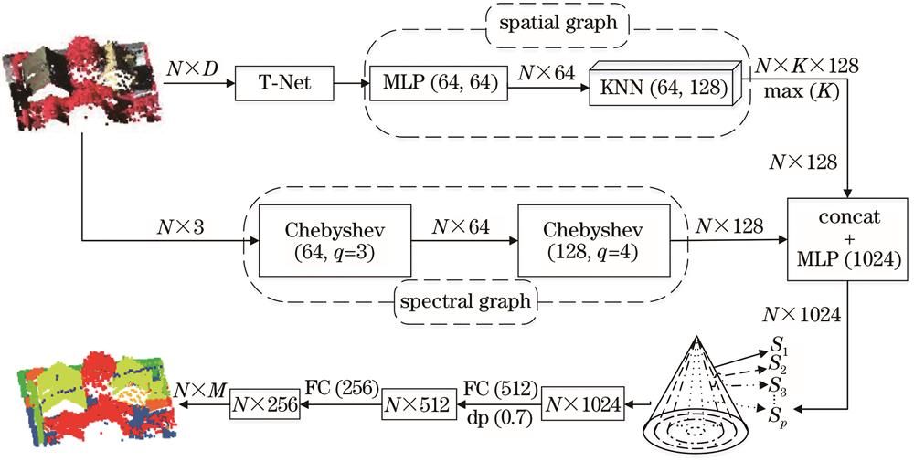
Fig. 1. Structure of the deep learning classification network
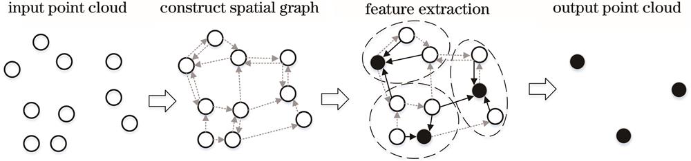
Fig. 2. Principle of the spatial domain graph convolution
Fig. 3. Schematic diagram of the KNN
Fig. 4. Central node information aggregated under different orders. (a) q=1; (b) q=2
Fig. 5. Training data and multispectral aerial image of corresponding region. (a) Point cloud; (b) aerial image
Fig. 6. Testing data and multispectral aerial images of corresponding region. (a) Point cloud; (b) aerial image
Fig. 7. Fusion result of point cloud data and spectral images. (a) Training data; (b) testing data
Fig. 8. Schematic diagram of multiscale sampling
Fig. 9. Testing data labels and classification results. (a) True label; (b) classification result of our method
Fig. 10. Error map of the classification result
Fig. 11. Error maps of classification results of different methods. (a) PointNet; (b) DGCNN; (c) PointNet++; (d) our method
Class | p_l | l_v | i_s | car | f_h | r_f | f_e | s_b | t_e |
---|
Training data | 546 | 180850 | 193723 | 4614 | 12070 | 152045 | 27250 | 47605 | 135173 | Testing data | 600 | 98690 | 101986 | 3708 | 7422 | 109048 | 11224 | 24818 | 54226 |
|
Table 1. Number of various classes points in Vaihingen data set
Class | p_l | l_v | i_s | car | f_h | r_f | f_e | s_b | t_e |
---|
p_l | 60.6 | 0.2 | 0.0 | 0.0 | 0.0 | 27.2 | 3.6 | 0.0 | 8.5 | l_v | 0.0 | 79.3 | 10.5 | 0.4 | 0.4 | 0.9 | 0.7 | 2.9 | 4.9 | i_s | 0.0 | 6.4 | 92.0 | 0.3 | 0.0 | 0.8 | 0.1 | 0.1 | 0.2 | car | 0.0 | 9.9 | 11.3 | 55.0 | 3.4 | 5.4 | 5.4 | 5.5 | 4.0 | f_h | 0.0 | 25.7 | 3.8 | 0.2 | 19.3 | 9.2 | 1.1 | 11.3 | 29.3 | r_f | 0.1 | 1.2 | 0.9 | 0.0 | 0.0 | 93.9 | 1.7 | 0.2 | 1.9 | f_e | 0.2 | 6.4 | 2.4 | 1.3 | 0.1 | 26.2 | 48.6 | 3.2 | 11.6 | s_b | 0.0 | 18.7 | 2.3 | 0.6 | 1.0 | 3.4 | 1.5 | 19.1 | 53.3 | t_e | 0.0 | 3.1 | 0.5 | 0.1 | 0.1 | 3.3 | 1.3 | 0.9 | 90.6 | Precision | 80.9 | 80.9 | 90.1 | 66.5 | 64.1 | 93.5 | 53.4 | 41.5 | 70.1 | Recall | 60.6 | 79.3 | 92.0 | 55.0 | 19.3 | 93.9 | 48.6 | 19.1 | 90.6 | F1 score | 69.3 | 80.1 | 91.0 | 60.2 | 29.6 | 93.7 | 50.9 | 26.1 | 79.1 |
|
Table 2. Confusion matrix and evaluation indexes of the classification result
Method | p_l | l_v | i_s | car | f_h | r_f | f_e | s_b | t_e | OA | F1 score |
---|
PointNet | 1.7 | 68.9 | 77.6 | 30.6 | 16.7 | 69.1 | 6.8 | 33.3 | 46.5 | 60.9 | 33.6 | DGCNN | 80.3 | 81.2 | 78.9 | 26.8 | 52.0 | 67.1 | 18.9 | 31.1 | 79.5 | 70.6 | 41.6 | PointNet++ | 71.5 | 72.0 | 90.0 | 68.3 | 16.7 | 74.0 | 38.4 | 39.2 | 52.7 | 73.6 | 50.1 | Ours | 80.9 | 80.9 | 90.1 | 66.5 | 64.1 | 93.5 | 53.4 | 41.5 | 70.1 | 84.3 | 64.4 |
|
Table 3. Quantitative evaluation index of different methods
Method | p_l | l_v | i_s | car | f_h | r_f | f_e | s_b | t_e | OA | F1 score |
---|
UM | 46.1 | 79.0 | 89.1 | 47.7 | 5.2 | 92.0 | 52.7 | 40.9 | 77.9 | 80.8 | 59.0 | WhuY3 | 37.1 | 81.4 | 90.1 | 63.4 | 23.9 | 93.4 | 47.5 | 39.9 | 78.0 | 82.3 | 61.6 | BIJ_W | 13.8 | 78.5 | 90.5 | 56.4 | 36.3 | 92.2 | 53.2 | 43.3 | 78.4 | 81.5 | 60.3 | RIT_1 | 37.5 | 77.9 | 91.5 | 73.4 | 18.0 | 94.0 | 49.3 | 45.9 | 82.5 | 81.6 | 63.3 | Ref.[21] | 68.4 | 80.2 | 91.4 | 78.1 | 37.0 | 93.0 | 60.5 | 46.0 | 79.4 | 82.2 | 70.7 | Ours | 69.3 | 80.1 | 91.0 | 60.2 | 29.6 | 93.7 | 50.9 | 26.1 | 79.1 | 84.3 | 64.4 |
|
Table 4. Classification results of our method and existing methods