• Matter and Radiation at Extremes
  • Vol. 6, Issue 6, 064402 (2021)
K. Burdonov1、2、3, A. Fazzini1, V. Lelasseux1, J. Albrecht1, P. Antici4, Y. Ayoul1, A. Beluze1, D. Cavanna1, T. Ceccotti5, M. Chabanis1, A. Chaleil6, S. N. Chen7, Z. Chen4, F. Consoli8, M. Cuciuc7, X. Davoine6, J. P. Delaneau1, E. d’Humières9, J.-L. Dubois9, C. Evrard1, E. Filippov0、3, A. Freneaux1, P. Forestier-Colleoni1, L. Gremillet6, V. Horny1、6, L. Lancia1, L. Lecherbourg6, N. Lebas1, A. Leblanc0, W. Ma0, L. Martin1, F. Negoita7, J.-L. Paillard1, D. Papadopoulos1, F. Perez1, S. Pikuz0, G. Qi0, F. Quéré5, L. Ranc0、1, P.-A. Söderström7, M. Scisciò8, S. Sun4, S. Vallières4, P. Wang0, W. Yao1、2, F. Mathieu1, P. Audebert1, and J. Fuchs1、a)
Author Affiliations
  • 0Joint Institute for High Temperatures, RAS, 125412 Moscow, Russia
  • 0Laboratoire Charles Fabry, Institut d’Optique Graduate School, CNRS, Université Paris-Saclay, 91127 Palaiseau Cedex, France
  • 0Laboratoire d’Optique Appliquée, Ecole Polytechnique–ENSTA–CNRS–Institut Polytechnique de Paris, Palaiseau, France
  • 0State Key Laboratory of Nuclear Physics and Technology, School of Physics, CAPT, Peking University, Beijing 100871, China
  • 1LULI–CNRS, CEA, Sorbonne Université, Ecole Polytechnique, Institut Polytechnique de Paris, F-91128 Palaiseau Cedex, France
  • 2Sorbonne Université, Observatoire de Paris, Université PSL, CNRS, LERMA, F-75005 Paris, France
  • 3IAP, Russian Academy of Sciences, 603155 Nizhny Novgorod, Russia
  • 4INRS-EMT, 1650, Boulevard Lionel-Boulet, Varennes, Québec J3X 1S2, Canada
  • 5Université Paris-Saclay, CEA, CNRS, LIDYL, 91191, Gif-sur-Yvette, France
  • 6Université Paris-Saclay, CEA, LMCE, 91680 Bruyères-le-Châtel, France
  • 7“Horia Hulubei” National Institute for Physics and Nuclear Engineering, 30 Reactorului Street, RO-077125 Bucharest-Magurele, Romania
  • 8ENEA, Fusion and Technologies for Nuclear Safety Department, C. R. Frascati, Via E. Fermi 45, 00044 Frascati, Italy
  • 9University of Bordeaux, Centre Lasers Intenses et Applications, CNRS, CEA, UMR 5107, F-33405 Talence, France
  • show less
    DOI: 10.1063/5.0065138 Cite this Article
    K. Burdonov, A. Fazzini, V. Lelasseux, J. Albrecht, P. Antici, Y. Ayoul, A. Beluze, D. Cavanna, T. Ceccotti, M. Chabanis, A. Chaleil, S. N. Chen, Z. Chen, F. Consoli, M. Cuciuc, X. Davoine, J. P. Delaneau, E. d’Humières, J.-L. Dubois, C. Evrard, E. Filippov, A. Freneaux, P. Forestier-Colleoni, L. Gremillet, V. Horny, L. Lancia, L. Lecherbourg, N. Lebas, A. Leblanc, W. Ma, L. Martin, F. Negoita, J.-L. Paillard, D. Papadopoulos, F. Perez, S. Pikuz, G. Qi, F. Quéré, L. Ranc, P.-A. Söderström, M. Scisciò, S. Sun, S. Vallières, P. Wang, W. Yao, F. Mathieu, P. Audebert, J. Fuchs. Characterization and performance of the Apollon short-focal-area facility following its commissioning at 1 PW level[J]. Matter and Radiation at Extremes, 2021, 6(6): 064402 Copy Citation Text show less
    Photographs of (a) the Apollon SFA and (b) the inside of the vacuum chamber. The off-axis parabola (OAP) that focuses the laser beam onto the target is shown. The various diagnostics used during the experiment are also labeled. The high-order harmonic generation (HHG) diagnostic serves to measure the spectrum of harmonics of the light emitted from the irradiated surface of solid targets. Protons stemming from the (nonirradiated) rear side of the solid targets are detected by a set of radiochromic film (RCF)11 stacks mounted on a motorized wheel. FSSR is the focusing spectrometer with spatial resolution. The label “R” on the Spectralon plate (a Lambertian scatter plate) stands for “reflection,” since this scatter plate allows the (specularly) reflected fraction of the laser beam to be visualized.
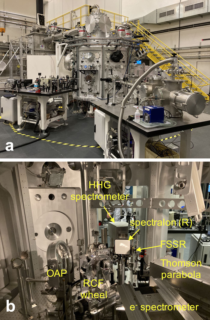
    Fig. 1. Photographs of (a) the Apollon SFA and (b) the inside of the vacuum chamber. The off-axis parabola (OAP) that focuses the laser beam onto the target is shown. The various diagnostics used during the experiment are also labeled. The high-order harmonic generation (HHG) diagnostic serves to measure the spectrum of harmonics of the light emitted from the irradiated surface of solid targets. Protons stemming from the (nonirradiated) rear side of the solid targets are detected by a set of radiochromic film (RCF)11 stacks mounted on a motorized wheel. FSSR is the focusing spectrometer with spatial resolution. The label “R” on the Spectralon plate (a Lambertian scatter plate) stands for “reflection,” since this scatter plate allows the (specularly) reflected fraction of the laser beam to be visualized.
    (a) Near-field beam profile at the output of the fourth amplification stage (out of five in total) operating at 38 J energy level. (b) Full-energy focal spot as measured in the interaction target after high-optical-quality neutral attenuation of the beam before compression. (c) Third-order cross-correlation intensity contrast measurement at the output of the first Ti:sapphire amplifier of the Apollon laser. The inset shows a typical Wizzler measurement of the compressed 24 fs pulses reaching the interaction chamber (solid line). The Fourier-transform-limited (i.e., diffraction-limited) pulse is plotted as a dashed line. (d) and (e) Oscilloscope screenshots showing the pulse contrast measurements using a fast photodiode at the output of the compressor. Two regimes are illustrated: (d) well-adjusted front-end system and nominal operation of the Apollon laser; (e) nonoptimized OPCPA (unstable injection) pump-signal instabilities have an impact on the end chain contrast. In both cases, the main pulse is saturated on purpose in order to see the weak prepulse ahead of it. Note that the peaked prepulse seen at 3 ns in (e) has the same amplitude as in (d). In (e), the vertical scale of the oscilloscope channel has been enlarged to better visualize the unstable behavior of the ASE in the last 3–4 ns before the laser peak. The purple trace in (d) and (e) is the facility trigger.
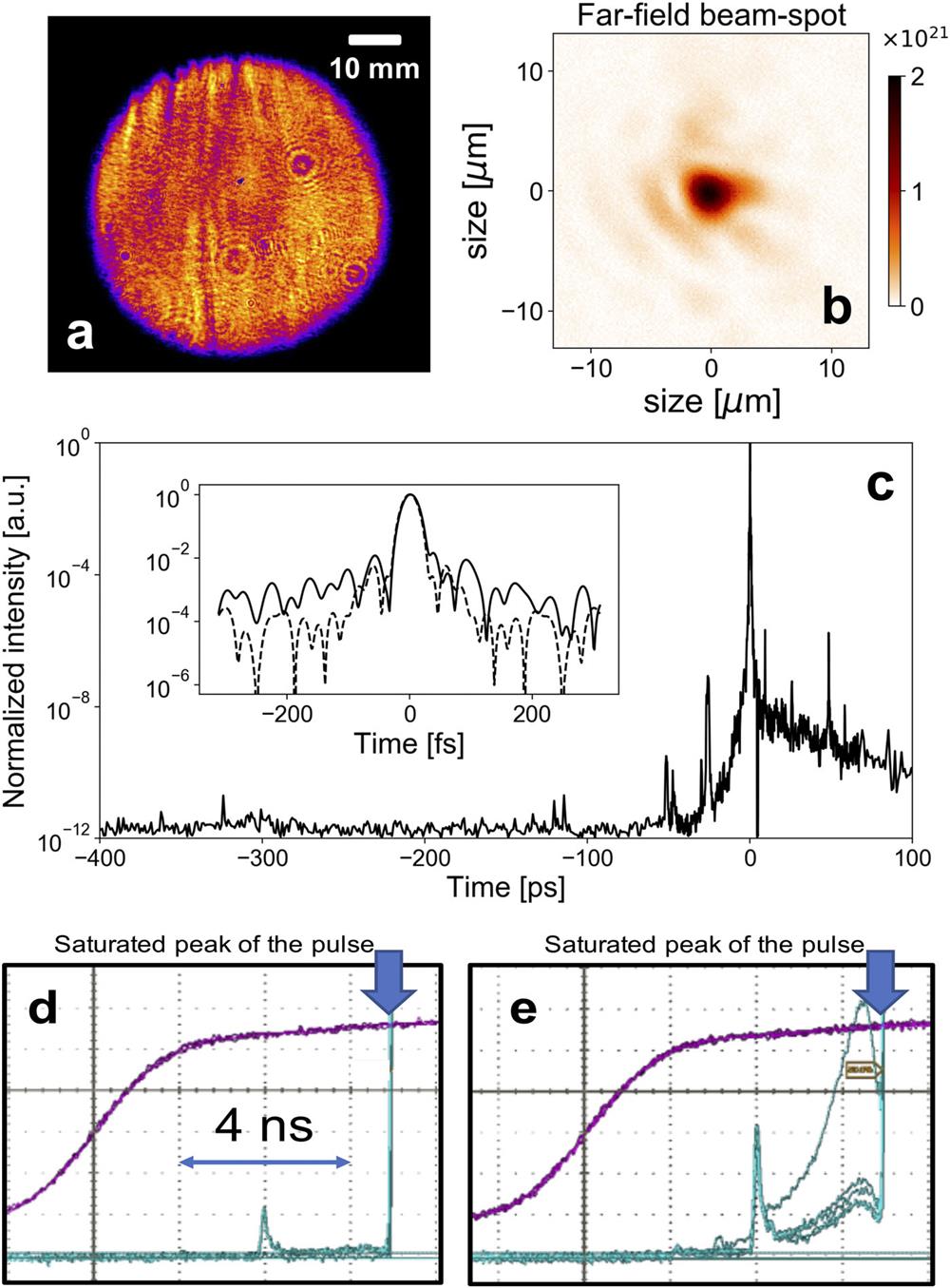
    Fig. 2. (a) Near-field beam profile at the output of the fourth amplification stage (out of five in total) operating at 38 J energy level. (b) Full-energy focal spot as measured in the interaction target after high-optical-quality neutral attenuation of the beam before compression. (c) Third-order cross-correlation intensity contrast measurement at the output of the first Ti:sapphire amplifier of the Apollon laser. The inset shows a typical Wizzler measurement of the compressed 24 fs pulses reaching the interaction chamber (solid line). The Fourier-transform-limited (i.e., diffraction-limited) pulse is plotted as a dashed line. (d) and (e) Oscilloscope screenshots showing the pulse contrast measurements using a fast photodiode at the output of the compressor. Two regimes are illustrated: (d) well-adjusted front-end system and nominal operation of the Apollon laser; (e) nonoptimized OPCPA (unstable injection) pump-signal instabilities have an impact on the end chain contrast. In both cases, the main pulse is saturated on purpose in order to see the weak prepulse ahead of it. Note that the peaked prepulse seen at 3 ns in (e) has the same amplitude as in (d). In (e), the vertical scale of the oscilloscope channel has been enlarged to better visualize the unstable behavior of the ASE in the last 3–4 ns before the laser peak. The purple trace in (d) and (e) is the facility trigger.
    (a) Laser focus beam-spot centroid motion with time; the dashed circle marks the diameter of the central peak of the laser spot, as can be seen in Fig. 2(b). (b) and (c) Corresponding weighted motion along the horizontal and vertical axes, respectively.
    Fig. 3. (a) Laser focus beam-spot centroid motion with time; the dashed circle marks the diameter of the central peak of the laser spot, as can be seen in Fig. 2(b). (b) and (c) Corresponding weighted motion along the horizontal and vertical axes, respectively.
    (a) Top-view schematic of the experimental setup. The red cone represents the focusing cone of the F2 beamline. (b) 3D rendering of the chamber bottom and target positioning system.
    Fig. 4. (a) Top-view schematic of the experimental setup. The red cone represents the focusing cone of the F2 beamline. (b) 3D rendering of the chamber bottom and target positioning system.
    (a) Target alignment procedure: the alignment beams produced by laser diodes coupled to beam expanders (Diode1 and Diode2) are transported inside the vacuum chamber by 100% reflective mirrors (M1 and M2) and are focused on the same point in space [the target chamber center (TCC), which is position 0 in (b)] by means of lenses (L1 and L2). The target can be adjusted in focus, i.e., back and forth along the main laser axis. The telescope, which is positioned outside the chamber, looks at the surface of the target with a high magnification. By scanning the target along the focus axis, we can observe that the two spots of the alignment beams are either overlapped [as in (c)] or separated [as in (d) and (e)]. The distance between the two spots depends on the target displacement from TCC, as shown in (b), where a positive direction corresponds to the target moving toward the laser-focusing OAP.
    Fig. 5. (a) Target alignment procedure: the alignment beams produced by laser diodes coupled to beam expanders (Diode1 and Diode2) are transported inside the vacuum chamber by 100% reflective mirrors (M1 and M2) and are focused on the same point in space [the target chamber center (TCC), which is position 0 in (b)] by means of lenses (L1 and L2). The target can be adjusted in focus, i.e., back and forth along the main laser axis. The telescope, which is positioned outside the chamber, looks at the surface of the target with a high magnification. By scanning the target along the focus axis, we can observe that the two spots of the alignment beams are either overlapped [as in (c)] or separated [as in (d) and (e)]. The distance between the two spots depends on the target displacement from TCC, as shown in (b), where a positive direction corresponds to the target moving toward the laser-focusing OAP.
    (a) and (b) Laser near-field images, captured after full amplification and before compression. (c) and (d) Images, captured by an imaging camera positioned outside the chamber, of the specularly reflected laser beam landing on the Spectralon plate after having irradiated (c) 10 µm and (d) 3 µm thick Al targets. The green arrow indicates the direction of laser propagation. The white rectangle in the bottom left of the images is the shadow of an object positioned between the target and the scatter plate, partially blocking the light on its way to the scatter plate. The top row shows poor contrast conditions and the bottom row good contrast conditions.
    Fig. 6. (a) and (b) Laser near-field images, captured after full amplification and before compression. (c) and (d) Images, captured by an imaging camera positioned outside the chamber, of the specularly reflected laser beam landing on the Spectralon plate after having irradiated (c) 10 µm and (d) 3 µm thick Al targets. The green arrow indicates the direction of laser propagation. The white rectangle in the bottom left of the images is the shadow of an object positioned between the target and the scatter plate, partially blocking the light on its way to the scatter plate. The top row shows poor contrast conditions and the bottom row good contrast conditions.
    Self-emission x-ray signals from the target front surface. (a) Images from (left) a Ti target, with poor laser contrast, and (right) an Al target, with good laser contrast. (b) Spectra from a thin Ti layer buried between plastic layers. (c) Al spectra obtained using the FSSR spectrometer, together with simulations performed using the PrismSPECT code. The simulated spectra are normalized to the experimental ones using the intensities of the Lyα and Heα lines. The offset in energy between the spectra obtained under good and poor contrast conditions is artificial and is plotted this way to allow comparison of the two spectra.
    Fig. 7. Self-emission x-ray signals from the target front surface. (a) Images from (left) a Ti target, with poor laser contrast, and (right) an Al target, with good laser contrast. (b) Spectra from a thin Ti layer buried between plastic layers. (c) Al spectra obtained using the FSSR spectrometer, together with simulations performed using the PrismSPECT code. The simulated spectra are normalized to the experimental ones using the intensities of the Lyα and Heα lines. The offset in energy between the spectra obtained under good and poor contrast conditions is artificial and is plotted this way to allow comparison of the two spectra.
    High-order harmonic spectrum measured during the commissioning experiment, using the F2 beamline of Apollon. The XUV beam in the specular axis resolved spectrally from ∼90 to ∼10 nm and, as can be seen in (a), resolved angularly in the range −30 to 30 mrad. (a) Raw image measured by imaging the MCP detector with a camera. (b) Angularly integrated signal between −10 and 10 mrad.
    Fig. 8. High-order harmonic spectrum measured during the commissioning experiment, using the F2 beamline of Apollon. The XUV beam in the specular axis resolved spectrally from ∼90 to ∼10 nm and, as can be seen in (a), resolved angularly in the range −30 to 30 mrad. (a) Raw image measured by imaging the MCP detector with a camera. (b) Angularly integrated signal between −10 and 10 mrad.
    (a) Schematic top view of Thomson parabola (TP). (b) Photograph of the back view with RadEye CMOS detectors. (c) Typical spectral image obtained in a single shot with the TP. One can clearly see the boundary between the two CMOS detectors that are mounted head to tail. The low-energy part of the spectrum has been intentionally cut by a thick Al filter, because it saturated the detector, since the number of particles increases exponentially toward low energies.
    Fig. 9. (a) Schematic top view of Thomson parabola (TP). (b) Photograph of the back view with RadEye CMOS detectors. (c) Typical spectral image obtained in a single shot with the TP. One can clearly see the boundary between the two CMOS detectors that are mounted head to tail. The low-energy part of the spectrum has been intentionally cut by a thick Al filter, because it saturated the detector, since the number of particles increases exponentially toward low energies.
    Maximum proton energies, as registered by RCFs and Thomson parabola, depending on the target thickness. The targets are plain Al foils.
    Fig. 10. Maximum proton energies, as registered by RCFs and Thomson parabola, depending on the target thickness. The targets are plain Al foils.
    (a) Photograph of the lateral panel of the electron spectrometer detector assembly, showing how the RadEye CMOS detectors are mounted on it. (b) Raw image of a recorded electron spectrum from a composite 20 nm Al + 23 µm polyethylene terephthalate (PET) target. For this particular shot, the distance from the TCC to the spectrometer entrance was 290 mm. (c) Hot-electron spectrum retrieved from the raw image [shown in (b)] and the corresponding Maxwellian distribution fit using an energy of 4 MeV.
    Fig. 11. (a) Photograph of the lateral panel of the electron spectrometer detector assembly, showing how the RadEye CMOS detectors are mounted on it. (b) Raw image of a recorded electron spectrum from a composite 20 nm Al + 23 µm polyethylene terephthalate (PET) target. For this particular shot, the distance from the TCC to the spectrometer entrance was 290 mm. (c) Hot-electron spectrum retrieved from the raw image [shown in (b)] and the corresponding Maxwellian distribution fit using an energy of 4 MeV.
    (a) Predicted number of events (as a function of time) produced in a boron-doped plastic scintillator of type EJ-254, placed at 6 m from the target, when exposed to the neutron spectrum shown by the dashed line in the inset. That neutron spectrum results from having a proton beam with maximum energy 28 MeV, also shown in the inset (full line) irradiating a Pb converter. The neutron generation in Pb is simulated using GEANT4. The events in the scintillator are simulated using the known cross-section in 10B (which decreases strongly when the incoming neutron energy increases), and the neutron spectrum (dashed line shown in the inset): starting at t = 0, there are no events, because there are no neutrons that have yet flown to the detector. As the neutron spectrum peaks around 1 MeV, and decreases for lower energies, this results in the events having a peak around 1 µs. (b) Actual time-of-flight chronogram recorded during the commissioning experiment, from a proton beam with maximum energy 28 MeV impinging on a 1 mm thick Pb converter. The signal is high at t = 0 owing to the gamma flash and the EMP. However, we notice a clear “bump” located at ∼1.5 µs, akin to what is expected based on the calculation shown in (a).
    Fig. 12. (a) Predicted number of events (as a function of time) produced in a boron-doped plastic scintillator of type EJ-254, placed at 6 m from the target, when exposed to the neutron spectrum shown by the dashed line in the inset. That neutron spectrum results from having a proton beam with maximum energy 28 MeV, also shown in the inset (full line) irradiating a Pb converter. The neutron generation in Pb is simulated using GEANT4. The events in the scintillator are simulated using the known cross-section in 10B (which decreases strongly when the incoming neutron energy increases), and the neutron spectrum (dashed line shown in the inset): starting at t = 0, there are no events, because there are no neutrons that have yet flown to the detector. As the neutron spectrum peaks around 1 MeV, and decreases for lower energies, this results in the events having a peak around 1 µs. (b) Actual time-of-flight chronogram recorded during the commissioning experiment, from a proton beam with maximum energy 28 MeV impinging on a 1 mm thick Pb converter. The signal is high at t = 0 owing to the gamma flash and the EMP. However, we notice a clear “bump” located at ∼1.5 µs, akin to what is expected based on the calculation shown in (a).
    OTR image collected at 1ω and emitted from the rear side of a 2 µm thick Al target. The image is larger than that of the focal spot shown in Fig. 2(b) owing to the intrinsic limited resolution of the f/6 imaging parabola.
    Fig. 13. OTR image collected at 1ω and emitted from the rear side of a 2 µm thick Al target. The image is larger than that of the focal spot shown in Fig. 2(b) owing to the intrinsic limited resolution of the f/6 imaging parabola.
    (a) Photograph of the electromagnetic field probes inside the target chamber: the D-dot probe is on the left behind the focusing parabola, and the B-dot probe is on the right. (b) Amplitude of the raw signals (expressed in volts and normalized to the laser energy) as a function of the laser focusing position on target (a motion in the positive direction means that the focusing parabola was moved closer to the target). (c) Temporal evolution of the electric (blue, D-dot) and magnetic (orange, B-dot) fields inside the target chamber. (d) Frequency spectra of the electric and magnetic fields displayed in (c).
    Fig. 14. (a) Photograph of the electromagnetic field probes inside the target chamber: the D-dot probe is on the left behind the focusing parabola, and the B-dot probe is on the right. (b) Amplitude of the raw signals (expressed in volts and normalized to the laser energy) as a function of the laser focusing position on target (a motion in the positive direction means that the focusing parabola was moved closer to the target). (c) Temporal evolution of the electric (blue, D-dot) and magnetic (orange, B-dot) fields inside the target chamber. (d) Frequency spectra of the electric and magnetic fields displayed in (c).
    K. Burdonov, A. Fazzini, V. Lelasseux, J. Albrecht, P. Antici, Y. Ayoul, A. Beluze, D. Cavanna, T. Ceccotti, M. Chabanis, A. Chaleil, S. N. Chen, Z. Chen, F. Consoli, M. Cuciuc, X. Davoine, J. P. Delaneau, E. d’Humières, J.-L. Dubois, C. Evrard, E. Filippov, A. Freneaux, P. Forestier-Colleoni, L. Gremillet, V. Horny, L. Lancia, L. Lecherbourg, N. Lebas, A. Leblanc, W. Ma, L. Martin, F. Negoita, J.-L. Paillard, D. Papadopoulos, F. Perez, S. Pikuz, G. Qi, F. Quéré, L. Ranc, P.-A. Söderström, M. Scisciò, S. Sun, S. Vallières, P. Wang, W. Yao, F. Mathieu, P. Audebert, J. Fuchs. Characterization and performance of the Apollon short-focal-area facility following its commissioning at 1 PW level[J]. Matter and Radiation at Extremes, 2021, 6(6): 064402
    Download Citation