Feature-enhanced fiber bundle imaging based on light field acquisition

Haogong Feng; Runze Zhu; Fei Xu

doi:10.3788/AI.2024.10002

Abstract

Optical fiber bundles frequently serve as crucial components in flexible miniature endoscopes, transmitting end-to-end images directly for medical and industrial applications. Each core usually acts as a single pixel, and the resolution of the image is limited by the core size and core spacing. We propose a method that exploits the hidden information embedded in the pattern within each core to break the limitation and obtain high-dimensional light field information and more features of the original image including edges, texture, and color. Intra-core patterns are mainly related to the spatial angle of captured light rays and the shape of the core. A convolutional neural network is used to accelerate the extraction of in-core features containing the light field information of the whole scene, achieve the transformation of in-core features to real details, and enhance invisible texture features and image colorization of fiber bundle images.

Keywords

deep learning fiber bundles image colorization image enhancement mode pattern

1. Introduction

Fiber optic endoscopes have demonstrated significant potential in biomedical and industrial manufacturing applications^[1–6] due to their high-temperature resistance, electromagnetic interference resistance, and bendability. An optical fiber bundle (FB) contains thousands of cores, each of which independently transmits light from the distal to the proximal, ensuring large information throughput in a small volume. Imaging resolution and image quality directly limit its application prospects. Smaller core sizes and core spacing mean higher spatial resolution, but weaker brightness and greater inter-core crosstalk^[7–9]. In the early years, researchers eliminated honeycomb noise by spatial and frequency domain filtering^[10,11], interpolation^[12], and a priori learning of FB patterns^[13,14], but no additional information was obtained to improve the spatial resolution. Mechanical scanning devices^[15] and optical elements^[16] were used to obtain multiple low-resolution images of different positions to combine high-resolution images, whose speed was limited by the scanning and alignment synthesis algorithms. Multiple wavelengths were utilized to improve imaging resolution^[17,18], but complex optical systems were required. A spatial light modulator has also been used to focus coherent light for scanning utilizing wavefront shaping^[19–21]. However, this method is sensitive to bending and temperature. In recent years, neural networks have been trained to learn mappings from restored FB images and estimated pseudo-ground truth (GT) from a microendoscope for the first time^[22]. The brightness mapping between the FB images and GT was constructed by a neural network (GARNN)^[23,24]. Learned high-resolution FB images were also used for medical diagnosis, and the network helped increase the classification accuracy from 90.8% to 95.6% for glioblastoma^[25]. In addition, with end-to-end deep-learning reconstruction algorithms, FB imaging systems are capable of reconstructing multispectral data with the integration of coding components^[26]. However, each core in FBs was regarded as one pixel in previous studies, and the information hidden inside the core is unexplored and unexploited, which limits its reconstruction resolution and information dimension.

Coding elements in optical pathways and computational frameworks are investigated to extract high-frequency information. A framework for computational imaging using different random binary masks and sparse-recovery algorithms in the FB endoscopy system was presented to reconstruct images with more resolved pixels in individual cores^[27,28]. Indeed, each core of the FB itself has unavailable hidden information including high-dimensional light field information because it usually contains a few modes. The proportion of different modes in the core is related to the light field captured at the distal^[29]. A digital aperture filtering approach used the FB as a light field sampling sensor to achieve a depth of field extension and three-dimensional (3D) light field imaging based on in-core modes^[30–32]. Light with different spatial incidence angles and different incidence positions is recorded by the FB in a pattern within the core, which implies more information than the intensity of individual pixels. If a mapping relationship between the in-core features and the distal multidimensional light field can be established, then the real image features at the distal end smaller than the core size can be reconstructed.

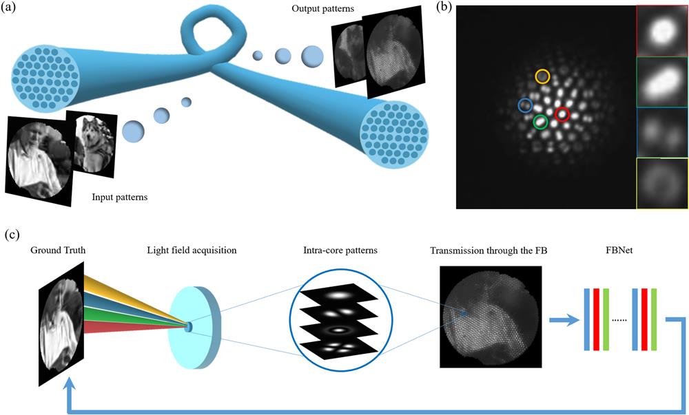
In this paper, we propose a method for restoring feature-enhanced FB images by the acquisition of the light field at the distal without extra elements in the probe and system. The edge, texture, and spectral features of the image in the real light field are encoded in the FB core pattern [in Fig. 1(c)]. Due to the random size and shape of their cores, it is time-consuming to implement computational decoding for each core individually. A generative adversarial neural network FBNet is used to learn a mapping from the pattern features in FB image cores to the GT high-frequency features and fill in the missing information (for a detailed description of the principle of operation). The enhanced natural grayscale images show a 12.7% improvement in the structural similarity index measure (SSIM) and a 14.1% improvement in peak signal-to-noise ratio (PSNR). Additionally, we facilitate the conversion of fiber endoscopic grayscale images to color images for the first time, enabling multispectral imaging without color filters. Intra-core intensity patterns enable the saturation of the reconstructed images close to the GT. The method fully utilizes the in-core modes to acquire and transmit incident multi-dimensional light field information, which greatly expands the transmission capacity of FBs and enriches the image content.

Figure 1.Schematic of light field acquisition and feature enhancement reconstruction using the FB. (a) Changes in the images after transmission through the FB, where a completely clear image is split into multiple core patterns by the fiber core. (b) A snapshot of the proximal face of the FB when it is illuminated with a fiber probe at the distal. The colored circles highlight the different patterns excited by different incidence angles. A partial zoom-in view is shown on the right. (c) The imaging process uses the FB to acquire the light field including light field acquisition, transmission, and reconstruction via FBNet.

2. Principle of Operation

2.1. Light Field Acquisition Using Fiber Bundles

The plenoptic function [ $P (θ, φ, λ, t, x, y, z)$ ] describing the light field contains the position $(x, y, z)$ of any point, any direction ( $θ, φ$ in polar coordinates), wavelength ( $λ$ ), and time ( $t$ ). The light field feature means more high-frequency detail for images. Figure 1(a) illustrates the real image split into several spots by the fiber core after passing through the FB, and Fig. 2(a) shows the end face of the FB and its spatial frequency feature map. In previous studies of FB image recovery, in-core patterns have usually been ignored. High-frequency information smaller than the core size is lost, corresponding to the frequency outside the red circle of the spatial frequency diagram below [in Fig. 2(a)]. The same intensity value collected on the sensor may correspond to a combination of multiple high-frequency features (edges, intensities, spectra, etc.) at the distal end [as shown in the upper part of Fig. 2(b)], which leads to a reconstruction bias of image details only through the intensity of each core.

Figure 2.Principle of light field acquisition using the FBs. (a) High-frequency light field information recorded in the core pattern. Up: spatial domain sampling of the FB. The yellow part corresponds to the fiber cores. Down: frequency domain sampling of the FB (given by the Fourier transform of the figure above). Low-frequency features are located in the center part of the image. Red circles correspond to the frequency of the core pitch size. (b) Sampling effect of different features smaller than the core size on the proximal end. Above: ignoring core features. Below: considering the in-core pattern. (c) On-axis Gaussian beam: the different color curves show the trend of the ratio of different excitation modes to the total incident power with an increasing angle of incidence. (d) Tilted Gaussian beam: the red curve shows the fundamental mode excitation efficiency as a function of a shift of a distance. (e) On-axis uniform beam: the red curve indicates the fundamental mode excitation efficiency as a function of the spot size of the beam and the modal.

FBs are used as light field acquisition sensors due to their large numerical aperture and few-mode properties within one core. A point light source of a few hundred nanometers in diameter is placed at the front of the FB to demonstrate that the light reaches the end face at different angles and excites different transmission modes (in different colors) in different cores, arising various patterns as shown in Fig. 1(b). That is, features smaller than the core size can be accurately distinguished by the patterns within the core [as shown in the lower part of Fig. 2(b)]. Nevertheless, it is difficult to recover different features only from the intensity values of a single fiber core. It is estimated that the number of transmission modes in each core is about 6–12 when the wavelength is in the range of 400–700 nm. The excitation of these modes is influenced by the spatial angle and position of the illumination on the end face.

According to the mode theory of optical fibers^[29], one core is assumed to be circular to facilitate the calculation of its corresponding light field. An accurate approximation can be used for weakly guiding fibers. $P_{l}$ is the power of one kind of linearly polarized mode and $P_{i}$ is the total incident power. $k$ is the propagation coefficient, $r_{0}$ is the modal spot size, and $ρ_{s}$ is the beam spot size. $n_{i}$ represents the refractive index and $θ_{i}$ represents the angle between the incident light and the fiber axis. The ratio of the power of each mode can be described as $\frac{P_{l}}{P_{i}} = 4 \frac{{(k ρ_{s} n_{i} θ_{i})}^{2 l}}{l!} {(\frac{r_{0} ρ_{s}}{r_{0}^{2} + ρ_{s}^{2}})}^{2 l + 2} \exp [- \frac{{(k ρ_{s} n_{i} θ_{i} r_{0})}^{2}}{r_{0}^{2} + ρ_{s}^{2}}] .$ (1)

According to Eq. (1), only the $l = 0$ modes are excited when the Gaussian beam is incident perpendicular to the end face at the center of the core. With the increase of the angle between the Gaussian beam and the fiber axis, higher order modes ( $l > 0$ ) are excited, and the power ratio of the fundamental mode gradually decreases as shown in Fig. 2(c). Figure 2(d) shows that the excitation efficiency of the fundamental mode [in Eq. (2)] is affected by a shift of a distance $r_{d}$ along the fiber axis of the offset Gaussian beam. When the Gaussian beam is replaced by the uniform beam with radius $ρ_{s}$ , the fraction of beam power exciting the fundamental mode can be expressed by Eq. (3). Fundamental mode and higher-order modes are excited simultaneously when the uniform beam is incident normally on the end face as shown in Fig. 2(e). The excitation efficiency of the fundamental mode is related to the radius of the beam, $\frac{P_{0}}{P_{i}} = {[2 \frac{r_{0} ρ_{s}}{(r_{0}^{2} + ρ_{s}^{2})}]}^{2} \exp [- \frac{r_{d}^{2}}{(r_{0}^{2} + ρ_{s}^{2})}],$ (2) $\frac{P_{0}}{P_{i}} = {(2 \frac{r_{0}}{ρ_{s}})}^{2} {[1 - \exp (- \frac{ρ_{s}^{2}}{2 r_{0}^{2}})]}^{2} .$ (3)

The image recorded on the image sensor contains a sampling of the incident light field from all the fiber cores in the form of mode patterns. Equation (4) describes the relationship between image features and the pattern of modes within the core on the sensor, where $Y_{P}$ denotes the arrangement of intensity values of pixels corresponding to a single core on the sensor. $P$ is the number of pixels, and $M$ denotes the number of modes that can be supported by the core. The image block corresponding to each fiber core at the far end is discretized into $N$ voxels, each with an intensity value of $I_{N}$ . The matrix $α$ represents the intensity contribution of different modes to different pixels, which can usually be calculated from the core size and wavelength. The rows represent the contribution of different modes to a single pixel on the sensor, and the columns represent the intensity distribution of different modes. The matrix $k$ represents the power share of different modes excited by each voxel and is obtained from Eq. (1) to Eq. (3). Based on the mode theory and the light field sampling of the fiber core, the power distributions of different mode fields are superimposed from the near-end shot. The high-frequency image features can be reconstructed once the matrix $α$ and matrix $k$ of each core are obtained, $(\begin{matrix} α_{11} & α_{12} & \dots & α_{1 M} \\ α_{21} & α_{22} & \dots & α_{2 M} \\ α_{31} & \dots & \dots & \dots \\ \dots & \dots & \dots & \dots \\ α_{P 1} & \dots & \dots & α_{PM} \end{matrix}) \times (\begin{matrix} k_{11} & k_{12} & \dots & k_{1 N} \\ k_{21} & k_{21} & \dots & k_{2 N} \\ \dots & \dots & \dots & \dots \\ k_{M 1} & \dots & \dots & k_{MN} \end{matrix}) \times (\begin{matrix} I_{1} \\ I_{2} \\ \dots \\ I_{N} \end{matrix}) = (\begin{matrix} Y_{1} \\ Y_{2} \\ \dots \\ Y_{P} \end{matrix}) .$ (4)

2.2. Neural Network Model for Optimal Reconstruction

By approximating the computation of individual cores, high-frequency optical fields were shown to be reconstructed by extracting hidden information within the cores. However, FBs have more than thousands or even tens of thousands of cores and are randomly shaped. Calculating and reconstructing each core individually affects the timeliness of the image. Therefore, a deep learning algorithm is applied to optimize the light field detail reconstruction process. The responses of different modes in each fiber core for different spatial locations are obtained during training. Our goal is to extract light field information from low-frequency sampled maps with in-core patterns to achieve reconstruction of distal real image details. In addition to eliminating the interference of foveal artifacts, conditional adversarial networks help fill in the blank information with the high-frequency information in previous learning-based work^[33–35]. Reasonable network structures and an objective function-based gradient descent method optimize the solution process of matrix $α$ and matrix $k$ in Sec. 2.1.

The network structure (FBNet) consists of two parts, where the generator ( $G$ ) is used to generate an output close to the real image, and the discriminator ( $D$ ) is used to classify the output with the real image as shown in Fig. 3(a). $x$ is the observed image, and $z$ is the random noise. $y$ is the output. $G (x)$ is the output of the $G$ . When the discriminator has difficulty distinguishing between the real graph and the generator output, the generator and discriminator are considered to have completed the training. U-FBNet and R-FBNet [as shown in Fig. S1 in the Supplementary Information (SI)] with different generators (U-Net^[36] and Resnet^[37]) were used separately to demonstrate that the intra-core pattern contributes to the reconstruction of high-frequency features. A Markovian discriminator (PatchGAN)^[33,34] tries to classify if each $N \times N$ patch in an image is real or fake, also facilitating the learning of intra-core detail information. Thus, the objective function of the adversarial network can be expressed as $L_{GAN} (G, D) = E_{x, y} [\log D (x, y)] + E_{x, z} {\log {1 - D [x, G (x, z)]}},$ (5)where $G$ tries to minimize this objective against an adversarial $D$ that tries to maximize it. Moreover, the generated image has to be closer to the real, so mixing the GAN objective with a more traditional loss $l_{1}$ is necessary, $L_{l_{1}} (G) = E_{x, y, z} [{‖ y - G (x, z) ‖}_{1}] .$ (6)

Figure 3.Neural network models and experimental setup. (a) Training procedure of the FBNet. The generator G learns to generate pseudo-real images in an attempt to fool the discriminator. Discriminator D learns to achieve classification between fake (synthesized by the generator) and real images. (b) FB image acquisition experimental setup diagram. The real image on the screen is displayed on the distal of the FB by a scaled combination of the lens ( $L_{1}$ , $f_{1} = 12 mm$ ) and objective ( ${OBJ}_{1}$ , $50 \times$ ). The pattern at the proximal of the FB is projected on the CMOS by a lens ( $L_{2}$ , $f_{2} = 30 mm$ ) and an objective ( ${OBJ}_{2}$ , $40 \times$ ).

Finally, the objective is $G^{*} = \arg \min_{G} \max_{D} L_{GAN} (G, D) + β L_{l_{1}} (G) .$ (7)

$β$ is a tunable weighting parameter that depends on the different kinds of samples, which is set to 50 in this paper. In the training, the classical GAN method of training a network is used, with one gradient descent step on $D$ followed by one step on $G$ . Minibatch SGD and the Adam solver are applied. The initial learning rate is set to 0.0002. More details about the network structure are available from Section S1 in the SI.

2.3. Experimental Setup and Data Acquisition

A FB image projection and acquisition system is set to directly acquire the real image and the image of the proximal end of the FB as shown in Fig. 3(b). The FB (FIGH-016-160S, Fujikura) used in this paper has an outer diameter of approximately 164 µm and a length of 0.5 m with 1491 cores. The cores are nearly circular and irregularly shaped, with a core spacing of approximately 3.2 µm. The GT images are displayed on computer monitors ( $2560 \times 1440$ , AOC) with a pixel pitch of 206 µm. Only an area of $128 \times 128$ in size is used to display the real image. The screen is projected onto the FB distal plane using a plano–convex lens ( $f_{2} = 30 mm$ , Thorlabs) and an objective ( $50 \times$ , LMPlanFi, Olympus). The reduction factor is approximately 175 times. The image transmitted through the FB is recorded by the complementary metal oxide semiconductor (CMOS) image sensor (panda 4.2, PCO) through a combination of objective ( $40 \times$ , Daheng) and plano–convex lenses ( $f_{1} = 12 mm$ , Thorlabs), magnified approximately 33.3 times. Each core pattern corresponds to about 40 or so pixels on the CMOS.

In the experiments, the public dataset, E-MINIST dataset, and ImageNet dataset^[38] are slightly optimized to fit the experimental requirements. The set of letters in the EMNIST dataset is used to create projection patterns. One of each of the 26 letters is selected, and four of them are stitched at random to form the new dataset C-letters with more various edges. Part of the ImageNet dataset is converted to grayscale to test for monochrome texture detail. The real data are displayed on the monitor at the time of acquisition, and the acquisition data containing core patterns are recorded directly by the magnification projection system, which is named the few-mode image dataset (FM). The corresponding reconstructed results using FBNet are called FM-X (where X can be U or R, respectively, corresponding to two different networks, U-FBNet and R-FBNet). As a comparison, the single-mode image dataset (SM) ignoring the mode patterns can also be obtained computationally. The positions of each core and the pixel coordinates of the region they occupy are first obtained by binarization and morphological processing.

Then the intensities of all pixels within each core are counted, and the average value is calculated. Finally, the intra-core Gaussian distribution of single-mode intensities is fitted based on the average value and the core radius, which is filled in the region to replace the original intra-core mode. Its reconstruction results are named SM-X (X is a placeholder, named in the same way as above). The reconstruction is operated on MATLAB and Python on a computer (CPU, Inter i3-10105) with GPU (NVIDIA GeForce RTX 3060) acceleration.

3. Results

3.1. Improvement of Edges

Image edges typically denote locally discontinuous features within the image. The genuine edges of the image are corrupted because the cladding portion of the FB is not transmitting light. Previous works only allow the acquisition of edge information at a resolution exceeding the core spacing. The resolution of the dataset C-letter at the FB end face is approximately 1.1 µm, significantly smaller than the core spacing. The lateral resolution at different spatial locations is affected by the random shape of the fiber core. SSIM and PSNR are employed for quantitative evaluation of image quality. Based on the networks mentioned in Sec. 2.2, the reconstruction process of the in-core pattern to real object detail maps is optimized, and the results are shown in Table 1.


		SSIM	PSNR	MOS
Interpolation	0.4119	12.1435	N/A
R-FBNet	SM-R	0.8963	24.4267	3.6667
	FM-R	0.9329	25.9967	4.4667
U-FBNet	SM-U	0.9092	24.5865	4.2000
	FM-U	0.9104	24.9419	4.3333

Table 1. Comparison of Testing Results for Boundary Features

View all Tables

The deep learning-based approach doubles the SSIM and PSNR compared to traditional interpolation methods. Various network structures are capable of achieving accurate reconstruction of most low-frequency information. However, compared to the method that ignores the in-core patterns (corresponding results SM-X), SSIM increases from 0.8963 to 0.9329, and PSNR increases from 24.4267 to 25.9967 when using the R-FBNet for image restoration of the FM. SSIM and PSNR also get a boost when the generator is the U-Net. Some of the test results are shown in Fig. 4 and Fig. S2 (in the SI). The original acquisition map (in the first row) is covered by the foveal noise of the FB itself, the image quality is degraded, and the edge information is corrupted. The red window is a zoom-in on the region of interest, where spatial features smaller than the core size excite higher-order modes in the fiber. The frequency spectrum in the third, sixth, and ninth columns is obtained using the Fourier transform. The similarity to the real image frequency information is marked on the image in white. Compared with interpolation methods, the overall visual effect of the reconstructed images obtained by the deep learning-based methods (SM and FM) is closer to the real map. For high-frequency information, the minor edge (within the orange circles) is more accurately recovered by the extraction of in-core features containing the light field information. Considering the percentage of high-frequency and low-frequency information in the images and their effects on SSIM and PSNR, it is a huge boost. In addition, mean opinion score (MOS) means perceiving, measuring, and evaluating changes and distortions in the information of two images with the same subject content in a subjective way, and judging the quality of the image by normalizing the scores of the observers. MOS studies involved 15 raters scoring all the restored images with an integral grade from 1 (worst) to 5 (best) based on fidelity and sharpness compared to the GT. The last row of Table 1 provides average MOS results. Images with intra-core patterns have better reconstructed visual quality. In this experiment, 2900 sheets from the C-letter dataset are utilized for training, 100 for validation, and 100 for testing. The GTs are displayed only in the green channel with 128 pixel × 128 pixel, and the FB images recorded are 768 pixel × 768 pixel in gray. The FM and SM are trained with their corresponding GTs by networks U-FBNet and R-FBNet, respectively, and the networks converge after 40 epochs in 36 and 88 min.

Figure 4.Results of training and testing of SM and FM using R-FBNet. The first row displays the original images recorded by the image sensor containing the mode patterns, their regions of interest, and the spatial frequency spectra. The results of reconstruction by the traditional interpolation method are shown in the second row. The third and fourth rows present the reconstruction results by R-FBNet for different datasets. Some boundary features are marked with orange circles. The ground truths (GTs) are listed in the last row as a comparison. The similarity coefficients of their spectrograms with the corresponding GTs are recorded in white.

3.2. Enhancement of Textural Features

Most scenes in nature vary in grayscale with more textural features. We adopt 9000 (7000 for training, 1000 for testing, and 1000 for validation) natural images from ImageNet^[36] as the GT to demonstrate that acquiring light field information with the FB helps in the reconstruction of 8-bit texture details. Multidimensional light field information, i.e., richer image content, is recorded and transmitted, although it is difficult for the naked eye to distinguish from FB patterns. Real images of different sizes are cropped to $128 \times 128$ and converted into a grayscale map. The $R$ channel of the on-screen image was set to grayscale map intensity while the $G$ and $B$ channels were set to 0. This considers that the wavelength can also have an effect on the structural pattern within the core. Similarly, we trained the direct acquisition map FM (with intra-core patterns) and SM (without intra-core patterns) images with R-FBNet and U-FBNet, respectively, until convergence.

The testing results are shown in Table 2. The average SSIM of the test images based on the FM images is 0.8051 (12.7% improvement compared to ignoring in-core patterns), and the average PSNR is 24.5879 (14.1% improvement compared to ignoring in-core patterns) when trained with the R-FBNet network. Similar results (SM-U: SSIM = 0.7355 and PSNR = 23.8912; FM-U: SSIM = 0.8076 and PSNR = 25.7332) were obtained when training with U-FBNet. The average MOS results agree with the SSIM and PSNR results listed in the last row of Table 2. Some of the results reconstructed through U-FBNet are presented in Fig. 5. The corresponding results using R-FBNet are shown in Fig. S3 in the SI. The reconstruction using FBNet (the third and the fourth rows) greatly improves the FB imaging quality compared to the direct acquisition map (the first row) and the conventional reconstruction map (the second row).


		SSIM	PSNR	MOS
R-FBNet	SM-R	0.7143	21.5485	3.6667
	FM-R	0.8051	24.5879	3.4333
U-FBNet	SM-U	0.7355	23.8912	2.9667
	FM-U	0.8076	25.7332	3.4667

Table 2. Comparison of Testing Results for Textural Features

View all Tables

Figure 5.Results of training and testing of the SM and FM for textural features through U-FBNet. The first, second, and last rows illustrate the raw acquisition maps, the reconstruction maps by traditional methods, and the real images. The third and fourth rows show the results of the reconstructions using the SM and FM as the dataset, respectively. The regions of interest are enlarged by the color window, corresponding to a real image size of about 40 µm at the distal.

It is difficult to discriminate these features effectively, even using deep learning techniques. FM-R and FM-U provide better enhancement than SM-R and SM-U for grayscale texture features within color windows such as a woman’s mouth (in the yellow window). The colored window area corresponds to a real image field of view of approximately 40 µm edge length, which is almost the same as the diameter of a hair. Our method is sufficient for endoscopic detection, cell imaging, etc. Due to the absence of sampling at the cladding at the front end of the FB, some distortion is inevitable. The network structure based on PatchGAN and the loss function containing loss L1 are employed to address this issue. Richer datasets and more optimized network structures may further overcome this problem.

3.3. Image Colorization

Usually, color image sensors have special arrays of color filters on their pixels. As each filter point can only pass one of the colors red, green, or blue, all pixels should have information about all three colors at the output. The two filtered color component values are made up in later algorithmic processing by interpolation, which distorts the directly acquired color image. In contrast, monochrome cameras give grayscale feedback for the color that is closer to the color-grayscale feedback of a real object. Its performance is superior to that of the color camera in terms of both luminous flux and detail. We provide a light-field-acquisition-based method for reconstructing color patterns from the grayscale patterns of FBs taken by monochrome cameras. In-core patterns influenced by light field information are shown to contribute to picture colorization. We select 9000 color images from the ImageNet^[36] dataset as a dataset, of which 7000 are used for training, 1000 for testing, and 1000 for validation. They are cropped to the same size of 32 pixel × 32 pixel and then enlarged to 128 pixel × 128 pixel for final display on the computer screen. Considering that the pattern structure is reconstructed while recovering the color information, we sacrifice some of the spatial resolution to color the directly captured grayscale images. The training set converges after 60 training epochs, taking a minimum of 132 min. The acquisition section is configured in Secs. 3.1 and 3.2.

Table 3 shows the results of the enhancement with U-FBNet and R-FBNet, respectively. The SSIM and PSNR of the color reconstruction were slightly lower compared to the projection and reconstruction of the single-channel image in Sec. 3.2. This is partly because the calculation of SSIM and PSNR for color images is influenced by the effect of color recovery, but also because the effective size of the image (32 pixel × 32 pixel) is reduced and a small error on a single pixel can have a significant impact. However, it is also true that the enhanced effect based on our method (FM-R: SSIM = 0.7096 and PSNR = 21.2329; FM-U: SSIM = 0.6487 and PSNR = 20.2941) is superior to that of enhancement by intensity within each core only (SM-R: SSIM = 0.6683 and PSNR = 20.6507; SM-U: SSIM = 0.6201 and PSNR = 20.1989). The average MOS results improve from 3.1333 to 3.4000 and from 3.3333 to 3.5333, respectively, when using the R-FBNet and U-FBNet. Figure 6 and Fig. S4 (in the SI) show partial results of testing. Surprisingly, the FBNet-based method accurately colors endoscopic grayscale images, which allows high dynamic range and high-resolution monochrome cameras to be used for color imaging scenes as well. For low-light imaging and measurements, the filterless multispectral acquisition provides greater luminous flux, increasing the accuracy of subsequent high-level vision tasks. Although the relationship between the in-core mode (FM-R) and color is difficult to perceive directly with the naked eye, the similarity of saturation of some reconstructed images to the GT has been marked with white numbers. Note that the reconstructed saturation maps of the red and blue channels are closer to that of GTs, and the green channel is less well-reproduced. One possible reason is that the magnified projection system is used at the far end and the lens chromatic aberration excites more higher-order patterns in the red and blue channels, making them easier to learn by the neural network. Another potential factor is that the green wavelength lies between the red and blue, and some patterns generated by the green incident light are learned as a superposition of the two incident light fields, red and blue, making the reconstructed map converge to gray. Theoretically, the reconstructed resolution and dimensionality of a color image are simultaneously affected by the number of modes within the fiber core. The use of hyperspectral data for training and more degrees of freedom of the developed system could further address the color crosstalk problem.


		SSIM	PSNR	MOS
R-FBNet	SM-R	0.6683	20.6507	3.1333
	FM-R	0.7096	21.2329	3.4000
U-FBNet	SM-U	0.6201	20.1989	3.3333
	FM-U	0.6487	20.2941	3.5333

Table 3. Testing Results for Image Colorization

View all Tables

Figure 6.Results of training and testing of the SM and FM for image colorization based on R-FBNet. The first row illustrates the raw SM and FM datasets used for image coloring. The colored maps and their saturation maps are shown in the second and third rows. The last row lists the GTs and their saturation graphs as a comparison. The white numbers indicate the similarity between the saturation of the reconstructed maps and the saturation of GTs.

4. Discussion

Based on the light field sampling characteristics of the FB and the potential information of multiple core channels, high-frequency detail information of the image at the distal end is extracted from the core pattern, which was often overlooked before. An evidence-based model is proposed, and deep learning methods are used to optimize the solving process to meet practical needs. Our enhancements improve over previous methods in edge reconstruction, texture recovery, and image colorization. Although other work may have obtained better performance metrics, this is influenced by the dataset and the fiber. When the in-core mode is ignored, the same-sized field of view on the detector can acquire a larger field of view at the far end, which has more information at lower frequencies. In contrast, the proportion of spatial frequencies lower than the core spacing is correspondingly reduced during reconstruction so that better reconstruction quality may be obtained. However, when the detection scene is small, the high-frequency details cannot be ignored. Our method can effectively reconstruct more high-frequency information from low-resolution samples. Fortunately, our method is equally applicable to improve the reconstruction quality of other algorithms.

The C-letters dataset with multiple simple edge features is used to demonstrate that spatial features smaller than the core pitch size can be reconstructed based on the learning of the pattern within the core. The reconstruction time is less than 0.1 s, much faster than traditional calibration calculation methods, which makes high-resolution video-rate imaging possible. However, measuring the improvement in resolution is difficult because the core size and shape are varied at different locations on the end face. Theoretically, the lateral spatial resolution of the far-end image tends to be infinitesimal, breaking through the limitations of the resolution of the imaging objective lenses L1 and L2 when the image sensor samples the intra-core patterns adequately. Small offsets cause the power share of different modes within the core to change, as shown in Fig. 2. However, the resolution of the reconstructed images is affected by the network structure and the number of network parameters. In practice, this value is also affected by the incident light field spectrum, FB inter-core coupling, transmission loss, and sensitivity of the near-end acquisition image sensor. Despite the utilization of incoherent light, the large curvature will cause some inter-core crosstalk and mode crosstalk, which will affect the image reconstruction. Although the image quality has been greatly improved by FBNet, the reconstruction of the ImageNet dataset is not as satisfactory as the C-letter dataset. This is because grayscale images are richer in image content, which is a huge test for the effective transmission capacity of the FB. In theory, the richness (resolution and color dimension) of the image reconstruction is limited by the number of modes supported for transmission within each fiber core. This may result in some image artifacts as shown in SM-R and SM-U that are well suppressed in FM-R and FM-U. In the future, more efficient network structures and richer datasets that meet the needs of the scenario will be considered to enhance the practical applications, including 3D imaging, high-speed imaging, and unsupervised learning. Additionally, the image colorization is based on the RGB channels, which is due to the storage format of the image in the computer. Higher spectral channel reconstruction is also applicable for this method but poses a higher challenge for the FB acquisition and transmission throughput. In addition, the attenuation of the light intensity of the real object also affects the effect of image coloring and needs to be further investigated.

5. Conclusion

The mode pattern within the core of a FB carries information about the distal excitation light field. Using the FB as an optical field sampling sensor rather than just an intensity transmission medium helps to capture multidimensional light fields, break the limitations of core spacing on the acquisition of detailed image features, and enhance information transmission capacity for a limited number of channels. We constructed a model for reconstructing the original image details based on low-frequency pattern maps and used deep-learning network structures to optimize the reconstruction process. Satisfactory results were obtained in applications such as image edge clarification, detail enhancement, and image coloring. High-frequency and multiwavelength light field information without light flux loss provides the possibility of low-light imaging, fluorescence imaging, and multispectral imaging in medical diagnostics, surgical navigation, and industrial measurements. Future plans for more application scenarios include training a more generalized network based on a few samples, 3D reconstruction of a single image, and real applications such as medical diagnosis and fluorescence imaging.

References

[1] A. Perperidis et al. Image computing for fibre-bundle endomicroscopy: a review. Med. Image Anal., 62, 101620(2020).

[2] R. Kuschmierz et al. Ultra-thin 3D lensless fiber endoscopy using diffractive optical elements and deep neural networks. Light Adv. Manuf., 2, 415(2021).

[3] Y. Du et al. Hybrid multimode-multicore fibre based holographic endoscope for deep-tissue neurophotonics. Light Adv. Manuf., 3, 1(2022).

[4] H. Feng et al. Endoscopic displacement measurement based on fiber optic bundles. Opt. Express, 30, 14948(2022).

[5] J. Sun et al. Quantitative phase imaging through an ultra-thin lensless fiber endoscope. Light Sci. Appl., 11, 204(2022).

[6] H. Feng et al. Lensless fiber imaging with long working distance based on active depth measurement. IEEE Trans. Instrum. Meas., 71, 7002507(2022).

[7] KL. Reichenbach, C. Xu. Numerical analysis of light propagation in image fibers or coherent fiber bundles. Opt. Express, 15, 2151(2007).

[8] X. Chen, KL. Reichenbach, C. Xu. Experimental and theoretical analysis of core-to-core coupling on fiber bundle imaging. Opt. Express, 16, 21598(2008).

[9] A. Perperidis et al. Characterization and modelling of inter-core coupling in coherent fiber bundles. Opt. Express, 25, 11932(2017).

[10] J. Han, J. Lee, J. U. Kang. Pixelation effect removal from fiber bundle probe based optical coherence tomography imaging. Opt. Express, 18, 7427(2010).

[11] M. Elter, S. Rupp, C. Winter. Physically motivated reconstruction of fiberscopic images. Proceedings of the International Conference on Pattern Recognition, 599(2006).

[12] P. Wang et al. Fiber pattern removal and image reconstruction method for snapshot mosaic hyperspectral endoscopic images. Biomed Opt. Express, 9, 780(2018).

[13] J. Han, SM. Yoon. Depixelation of coherent fiber bundle endos-copy based on learning patterns of image prior. Opt. Lett., 36, 3212(2011).

[14] J. Shao et al. Resolution enhancement for fiber bundle imaging using maximum a posteriori estimation. Opt. Lett., 43, 1906(2018).

[15] Y. Chang et al. Compact high-resolution endomicroscopy based on fiber bundles and image stitching. Opt. Lett., 43, 4168(2018).

[16] SJ. Miller et al. Targeted detection of murine colonic dysplasia in vivo with flexible multispectral scanning fiber endoscopy. J. Biomed Opt., 17, 021103(2012).

[17] N. Krstajic et al. Two-color widefield fluorescence microendoscopy enables multiplexed molecular imaging in the alveolar space of human lung tissue. J. Biomed Opt., 21, 1(2016).

[18] R. French, S. Gigan. Snapshot fiber spectral imaging using speckle correlations and compressive sensing. Opt. Express, 26, 32302(2018).

[19] M. Plöschner, T. Tyc, T. Čižmár. Seeing through chaos in multi-mode fibres. Nat. Photonics, 9, 529(2015).

[20] E. R. Andresen et al. Toward endoscopes with no distal optics: video-rate scanning microscopy through a fiber bundle. Opt. Lett., 38, 609(2013).

[21] E. Scharf et al. Video-rate lensless endoscope with self-calibration using wavefront shaping. Opt. Lett., 45, 3629(2020).

[22] D. Ravì et al. Effective deep learning training for single-image super-resolution in endomicroscopy exploiting video-registration-based reconstruction. Int. J. Comput. Assist. Radiol. Surg., 13, 917(2018).

[23] J. Shao et al. Fiber bundle image restoration using deep learning. Opt. Lett., 44, 1080(2019).

[24] J. Shao et al. Fiber bundle imaging resolution enhancement using deep learning. Opt. Express, 27, 15880(2019).

[25] J. Wu et al. Learned end-to-end high-resolution lensless fiber imaging toward intraoperative real-time cancer diagnosis(2022).

[26] Z. Meng et al. Snapshot multispectral endomicroscopy. Opt. Lett., 45, 3897(2020).

[27] J. P. Dumas et al. Computational endoscopy—a framework for improving spatial resolution in fiber bundle imaging. Opt. Lett., 44, 3968(2019).

[28] J. Shin et al. A minimally invasive lens-free computational microendoscope. Sci. Adv., 5, eaaw5595(2019).

[29] K. Okamoto. Fundamentals of Optical Waveguides(2021).

[30] M. Levoy et al. Light field microscopy. ACM Transact Graph, 25, 924(2006).

[31] A. Orth et al. Extended depth of field imaging through multicore optical fibers. Opt. Express, 26, 6407(2018).

[32] A. Orth et al. Optical fiber bundles: ultra-slim light field imaging probes. Sci. Adv., 5, 1(2019).

[33] P. Isola et al. Image-to-image translation with conditional adversarial networks. Proceedings of the IEEE Conference on Computer Vision and Pattern Recognition, 1125(2017).

[34] JY. Zhu et al. Unpaired image-to-image translation using cycle-consistent adversarial networks. Proceedings of the IEEE International Conference on Computer Vision, 2223(2017).

[35] C. Ledig et al. Photo-realistic single image super-resolution using a generative adversarial network. Proceedings of the IEEE Conference on Computer Vision and Pattern Recognition, 4681(2017).

[36] O. Ronneberger, P. Fischer, T. Brox. U-net: Convolutional net-works for biomedical image segmentation. Proceedings of the International Conference on Medical Image Computing and Computer-Assisted Intervention, 234(2015).

[37] K. He et al. Deep residual learning for image recognition. Proceedings of the IEEE conference on computer vision and pattern recognition, 770(2016).

[38] J. Deng et al. ImageNet: a large-scale hierarchical image database. Proceedings of the IEEE Conference on Computer Vision and Pattern Recognition, 248(2009).