
Sunny Howard, Jannik Esslinger, Robin H. W. Wang, Peter Norreys, Andreas Döpp, "Hyperspectral compressive wavefront sensing," High Power Laser Sci. Eng. 11, 03000e32 (2023)
- High Power Laser Science and Engineering
- Vol. 11, Issue 3, 03000e32 (2023)
Abstract
Keywords
1 Introduction
Ultrashort laser pulses possess a necessarily broad spectral bandwidth[1]. The chromatic properties of the optical elements that are used for the generation or application of such pulses can then create relations between the spatial and temporal profiles, called spatio-temporal couplings (STCs)[2]. These phenomena can lead to a variety of effects including, for example, the broadening of a focused laser pulse either spatially or temporally, thereby reducing its peak intensity[3]. Deliberately introduced STCs can lead to exotic light pulses that behave very differently from ‘normal’ pulses. An example of this is the so-called flying focus[4] with its potential application in laser-driven wakefield accelerators[5] and orbital angular momentum beams[6]. Universally, the expansion in the applications of ultrafast laser pulses has exacerbated the need for a robust way to measure their properties.
To resolve STCs, one must gain wavefront information over the 3D hypercube (
Inspired by recent progress in machine-learning-based laser science[13], here we present the concept for a single-shot method that utilizes compressed sensing (CS) to resolve the wavefront in both the spectral and spatial domains. The paper is structured as follows. In Section 2 we will discuss the wavefront sensor and in Section 3 we introduce snapshot compressive imaging (SCI) as a way to expand the wavefront sensor to measuring multiple colours at once. Our implementation is based on deep unrolling, which yields high performance in both reconstruction fidelity and speed, as required for use as a real-time diagnostic. Section 4 provides a thorough description of all neural network architectures used, and Section 5 contains a description of how training data was generated, before Section 6 displays the results of the proposed method.
Sign up for High Power Laser Science and Engineering TOC. Get the latest issue of High Power Laser Science and Engineering delivered right to you!Sign up now
2 Wavefront sensing
The wavefront sensor that was simulated in this example was a quadriwave lateral shearing interferometer (QWLSI), which is known for its high resolution and reconstruction fidelity. Nonetheless, our method can in general be applied to any kind of wavefront retrieval technique, including the popular Shack–Hartmann sensor or multi-plane techniques, such as Gerchberg–Saxton phase retrieval.
A lateral shearing interferometer (LSI) measures the spatially varying phase of a light beam, and was first applied to the measurement of ultrashort laser pulses in the late 1990s[14]. The LSI works by creating multiple copies of the laser pulse and shearing them laterally relative to each other before their interference pattern is captured on a sensor. Due to the shear, information about the spatial gradient of the wavefront is encoded in the interferogram. This can then be extracted using Fourier filtering[15] and stitched together to form the wavefront via methods such as modal reconstruction[16] or Fourier integration[17]. The most popular implementation is the aforementioned QWLSI. By generating and shearing four (
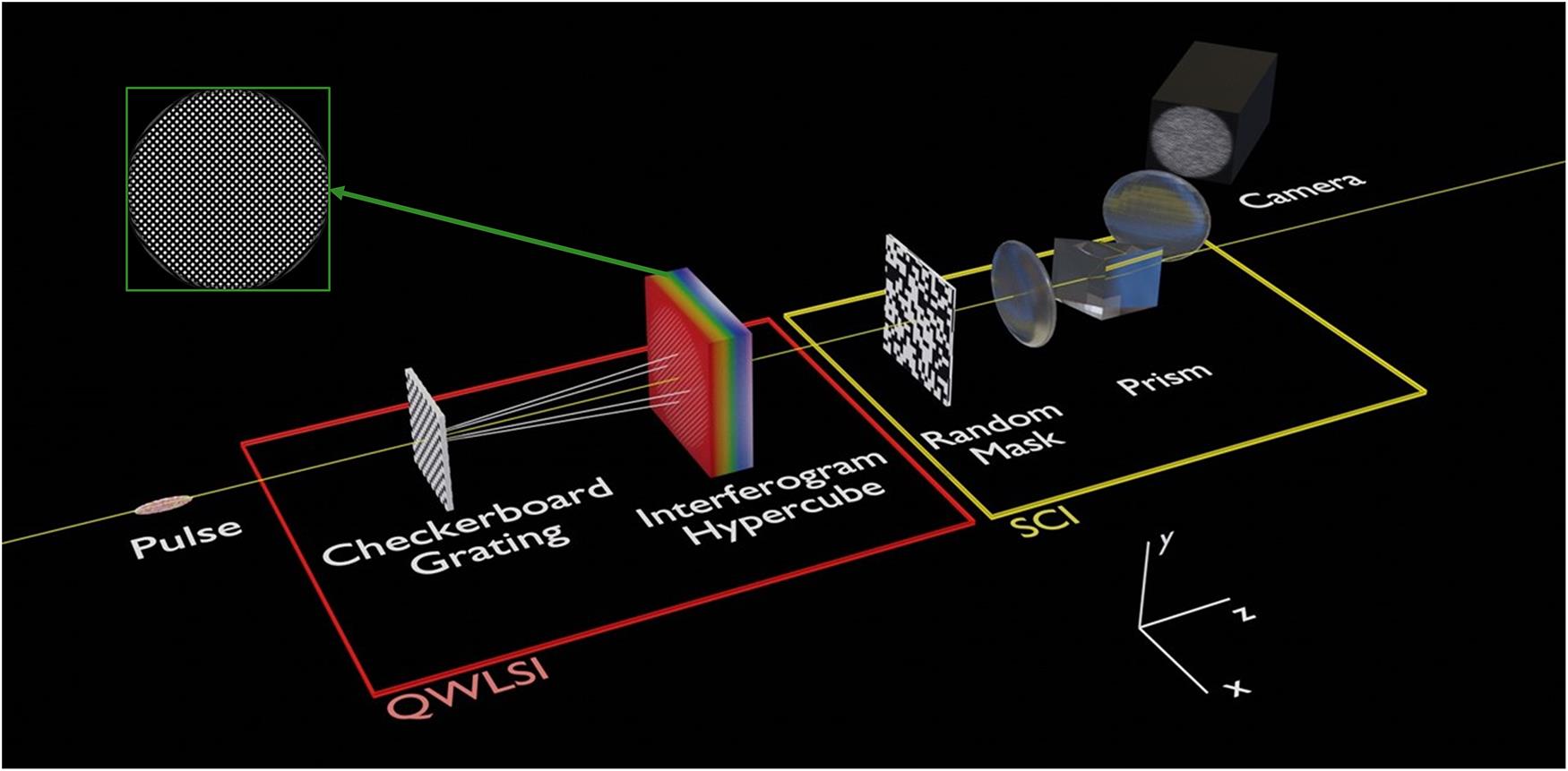
Figure 1.Schematic of the experimental setup that was simulated. The pulse first travels through a quadriwave lateral shearing interferometer, yielding a hypercube of interferograms, a slice of which is shown in the green box. The hypercube is then passed through a CASSI setup. This consists of a random mask and a relay system encompassing a prism, before the coded shot is captured with the camera. This diagram is not to scale.
2.1 QWLSI simulation
A physical implementation of the QWLSI usually consists of a phase grating with ‘pixels’ of alternating phase arranged in a checkerboard pattern[18], which leads to dominant diffraction in
The pulse is copied four times, and each copy’s field is propagated to the detector plane according to the following rules. Note that for brevity, when the
2.1.1 Propagation
Considering the jth copy has travelled a distance
In a QWLSI, the poloidal angles are
The resulting electric field of the copy is as follows:
2.1.2 Tilt
As diffraction occurs at an angle
Combining these two effects and summing over copies, we obtain the final changes to the field:
At the Talbot self-imaging plane,
In other applications one would collapse the cube onto a sensor at this point; however, this would eliminate the chance of retrieving the spectrally resolved phase. Instead, as discussed in Section 3, we use SCI to aid in the capturing of the cube.
2.2 Wavefront reconstruction
Once the interferogram is captured, one must extract the wavefront. As previously mentioned, current reconstruction methods usually involve multiple steps, that is, extracting the gradients, integrating and stitching them together. This can be a time-consuming process, especially in a hyperspectral setting where the reconstruction has to be done for every channel. To address this problem, we present a deep learning approach to wavefront reconstruction for the LSI. While similar work has been done in the context of Shack–Hartmann sensors[19,20], this is the first application of deep learning to LSI reconstruction, to the best of our knowledge. The network that was used will be discussed in Section 4.
3 Snapshot compressive imaging
CS describes the highly efficient acquisition of a sparse signal from fewer samples than would classically be required according to the Nyquist theorem by utilizing optimization methods to solve underdetermined equations. SCI is an example of CS, capturing 3D data on a 2D sensor in a single shot.
Fundamentally, there are two requirements to be fulfilled for CS to work. Firstly, the signal must be sparse on some basis and, secondly, the signal must be sampled on the basis that it is incoherent with respect to the sparse basis[21]. The first condition was hypothesized to be satisfied given the fact that laser wavefronts are known to be well-expressed with a few coefficients of the Zernike basis. When one does not have prior knowledge about which basis the signal is sparse on, the second condition is often solved by performing random sampling. Whilst being trivial for 2D data, in the context of SCI it is challenging, as the 3D hypercube must be randomly sampled onto a 2D sensor. To do so, nearly all research in this area uses hardware based on the coded aperture snapshot compressive imaging (CASSI) system[22,23].
3.1 CASSI
The hypercube is first imaged onto a coded aperture. This is a binary random mask with each pixel transmitting either 100% or 0% of the light. The cube is then also passed through some dispersive media, for example, a prism or grating, before being captured by a sensor, resulting in what is known as the coded shot. The effect of this optical system is that when the hypercube reaches the detector plane, each spectral channel is encoded with a different coded aperture, thereby approximating random sampling across the whole cube. It is then possible for a reconstruction algorithm to retrieve the cube. A diagram of a CASSI system is shown in the yellow box in Figure 1, with an example of a coded shot for an interferogram hypercube shown on the far left of Figure 3. The setup can easily be simulated by multiplying the cube by the mask, then shifting the channels of the cube according to the amount of (angular) dispersion imparted onto them, and finally summing over the spectral axis.
Mathematically, the CASSI system discussed above is summarized into a matrix
In order to reconstruct
The first term on the right-hand side is labelled the data term, and enforces that the hypercube must match the coded shot when captured. This alone would be an underdetermined system, so a regularization term, parameterized by
Most methods that have been developed to solve this non-convex equation can be sorted into two classes: iterative algorithms or end-to-end neural networks. The former offers good generalization but lacks abstraction capability and is slow, whilst deep nets are fast and have been shown to learn almost any function, but can be prone to overfitting[24]. A middle ground that offers state-of-the-art performance is deep unrolling.
3.2 Deep unrolling
While an end-to-end neural net would attempt to solve Equation (5) directly, if it were possible to split the equation, the data term can actually be solved analytically. This is desirable as it alleviates the abstraction needed to be done by the network, resulting in greater generalization and better parameter efficiency[25]. To perform such a separation, half quadratic splitting is employed. Firstly, an auxiliary variable
Here,
The benefit of this problem formulation is that it is then possible to split Equation (7) into two minimization sub-problems in
Equation (9) is a convex equation and can be solved via a conjugate gradient algorithm, which provides better stability than solving analytically. On the right-hand side of Equation (8),
The deep unrolling process is shown in Figure 2(b) panel (i). Firstly
![]()
Figure 2.A diagram showing the full reconstruction process of the wavefront from the coded shot. (a) A flow chart of the reconstruction process. (b) (i) The deep unrolling process, where sub-problems ① and ② are solved recursively for 10 iterations. Also shown is the neural network structure used to represent  . (ii) The training curve for the deep unrolling algorithm. Plotted is the training and validation PSNR for the 3D ResUNet prior that was used, as well as the validation score for a local–nonlocal prior. Here is demonstrated the superior power of 3D convolutions in this setting. (i) The network design for the Xception-LSI network. The Xception* block represents that the last two layers were stripped from the conventional Xception network. (c) (ii) The training curve for Xception-LSI for training and validation sets, with the loss shown in log mean squared error. Also plotted is the validation loss when further training the model on the deep unrolling reconstruction of the data (transfer).
4 Network architecture
This section contains the architectures of the neural networks that were used. They will be discussed in the order they are used in the reconstruction process, which is displayed in the flow chart of Figure 2(a). Firstly, the deep unrolling algorithm performs reconstruction of the interferogram hypercube from the coded shot, and secondly another network, Xception-LSI, reconstructs the spatial-spectral wavefront from the hypercube.
4.1 Deep unrolling regularizer
As previously discussed, the neural network,
4.2 Xception-LSI
A wavefront retrieval network was developed that takes a single spectral channel QWLSI interferogram and predicts the spatial wavefront in terms of Zernike coefficients. The network is based on the Xception network[29], but as the original 71-layer network is designed for classification, some changes were made to adapt Xception to our application. Firstly, the final two layers were removed. A max pool layer and a convolutional layer were added to shrink the output in the spatial and spectral dimensions, respectively. Dropout was applied before using three dense layers with 1000, 500 and 100 nodes using the ReLu activation function[30]. The output layer consists of 15 nodes with linear activation, corresponding to the number of Zernike coefficients to predict. We name the network Xception-LSI, and it can be seen in Figure 2(c) panel (i).
5 Training data generation
To represent the initial pulse, a total of 300 cubes were generated with dimensions
Each cube was then processed according to Figure 1. Firstly, it was passed through the QWLSI simulation (see Section 2.1), yielding a hypercube of interferograms – these are the training labels for the deep unrolling algorithm. This hypercube was then passed through the SCI simulation, yielding a coded shot – the training data. The wavefront was reconstructed via the process in Figure 2(a). The interferogram hypercube was reconstructed via deep unrolling, before being passed into the Xception-LSI network to predict the spectral Zernike coefficients.
The pitch of the LSI was set to
Before being passed through the deep unrolling network, the cubes and coded shots were split spatially into 64
The Xception-LSI network was fed individual channels of the ground truth interferogram hypercubes and predicted Zernike coefficients. Normal random noise (
6 Results and discussion
6.1 Snapshot compressive imaging
Crucial to this method’s success is the SCI reconstruction of the hypercube of interferograms. As can be seen from the green box of Figure 1, the image slices are modulated and appear as spot patterns. As a result, the images do not exhibit the same sparsity in, for example, the wavelet domain, as most natural images used in SCI research do. Because of this, there was uncertainty in whether it would be possible to recover the cube.
Here it is demonstrated that it is indeed possible to reconstruct such modulated signals with SCI. The training curve can be seen in Figure 2(b) panel (ii). Also plotted is the validation loss when a local–nonlocal prior[31], which is state-of-the-art for natural images, was used. One sees that when both architectures were used with 10 iterations of unrolling, the 3D convolutional model achieved a far superior peak signal-to-noise ratio (PSNR) of 36 compared to 29. Furthermore, it contains approximately 45% fewer parameters.
6.2 QWLSI
In order to reconstruct the wavefront for a full hypercube, each spectral channel is fed through the network sequentially. After training, the final mean squared error on the ground truth test set was
6.3 Hyperspectral compressive wavefront sensing
An example of the full reconstruction process, from coded shot to spatial-spectral wavefront, is displayed in Figure 3. It is apparent that the deep unrolling network was able to accurately reconstruct the interferogram hypercube, and the Xception-LSI network was able to reconstruct the wavefront.
![]()
Figure 3.Example results of the reconstruction process. (a) An example of the coded shot, along with a zoomed section. (b) Deep unrolling reconstruction of the interferogram hypercube in the same zoomed section at different wavelength slices. (c) The Xception-LSI reconstruction of the spatio-spectral wavefront displayed in terms of Zernike coefficients, where the
7 Summary and outlook
In this report we have demonstrated the possibility of combining a wavefront sensor with SCI in order to achieve a single-shot measurement of the spatial-spectral phase. Crucially, it has been shown that SCI has the ability to reconstruct modulated signals, such as those produced by a QWLSI.
A natural progression to this study is to realize the results in an experimental setting, where challenges arise from the more complicated dispersion, transfer functions and noise. Other further work could include extending the deep learning LSI analysis to the hyperspectral setting. By passing the network a hypercube of interferograms, rather than individual slices, it may be possible to exploit spectral correlations in order to improve accuracy and detect STCs more easily. Also, work can be done on testing the model with a more varied set of Zernike polynomials. Finally, there has been recent interest in the possibility of spreading phase contrast imaging to a hyperspectral setting. However, current methods take many seconds to capture a hypercube of phase[32]. The proposed method would be able to collect information with higher spectral resolution in a single shot, allowing for dynamic events to be recorded hyperspectrally.
References
[1] S. Jolly, O. Gobert, F. Quere. J. Opt., 22, 103501(2020).
[2] A. Jeandet, S. W. Jolly, A. Borot, B. Bussière, P. Dumont, J. Gautier, O. Gobert, J.-P. Goddet, A. Gonsalves, A. Irman, W. P. Leemans, R. Lopez-Martens, G. Mennerat, K. Nakamura, M. Ouillé, G. Pariente, M. Pittman, T. Püschel, F. Sanson, F. Sylla, C. Thaury, K. Zeil, F. Quéré. Opt. Express, 30, 3262(2022).
[3] C. Bourassin-Bouchet, M. Stephens, S. de Rossi, F. Delmotte, P. Chavel. Opt. Express, 19, 17357(2011).
[4] D. H. Froula, J. P. Palastro, D. Turnbull, A. Davies, L. Nguyen, A. Howard, D. Ramsey, P. Franke, S.-W. Bahk, I. A. Begishev, R. Boni, J. Bromage, S. Bucht, R. K. Follett, D. Haberberger, G. W. Jenkins, J. Katz, T. J. Kessler, J. L. Shaw, J. Vieira. Phys. Plasmas, 26, 032109(2019).
[5] C. Caizergues, S. Smartsev, V. Malka, C. Thaury. Nat. Photonics, 14, 475(2020).
[6] R. Aboushelbaya. Orbital angular momentum in high-intensity laser interactions(2021).
[7] P. Bowlan, P. Gabolde, A. Shreenath, K. McGresham, R. Trebino, S. Akturk. Opt. Express, 14, 11892(2006).
[8] M. López-Ripa, I. J. Sola, B. Alonso. Photon. Res., 10, 922(2022).
[9] S. L. Cousin, J. M. Bueno, N. Forget, D. R. Austin, J. Biegert. Opt. Lett., 37, 3291(2012).
[11] G. Pariente, V. Gallet, A. Borot, O. Gobert, F. Quéré. Nat. Photonics, 10, 547(2016).
[12] P. Gabolde, R. Trebino. Opt. Express, 14, 11460(2006).
[14] J.-C. Chanteloup, F. Druon, M. Nantel, A. Maksimchuk, G. Mourou. Opt. Lett., 23, 621(1998).
[15] M. Takeda, H. Ina, S. Kobayashi. J. Opt. Soc. Am., 72, 156(1982).
[16] F. Dai, F. Tang, X. Wang, O. Sasaki, P. Feng. Appl. Opt., 51, 5028(2012).
[17] S. Velghe, J. Primot, N. Guérineau, M. Cohen, B. Wattellier. Opt. Lett., 30, 245(2005).
[18] S. Velghe, J. Primot, N. Guérineau, R. Haïdar, S. Demoustier, M. Cohen, B. Wattellier. Proc. SPIE, 6292(2006).
[19] L. Hu, S. Hu, W. Gong, K. Si. Opt. Express, 27, 33504(2019).
[20] L. Hu, S. Hu, W. Gong, K. Si. Opt. Lett., 45, 3741(2020).
[21] E. J. Candes. Comptes Rendus Math, 346, 589(2008).
[22] M. E. Gehm, R. John, D. J. Brady, R. M. Willett, T. J. Schulz. Opt. Express, 15, 14013(2007).
[23] A. Wagadarikar, R. John, R. Willett, D. Brady. Appl. Opt., 47, B44(2008).
[24] X. Yuan, D. J. Brady, A. K. Katsaggelos. , , and , IEEE Signal Process. Mag. , 65 ()., 38(2021).
[25] V. Monga, Y. Li, Y. C. Eldar. , , and , IEEE Signal Process. Mag. , 18 (2021)., 38.
[26] Z. Wu, J. Zhang, C. Mou. , , and , ().(2021). arXiv:2109.06548
[27] Z. Zhang, Q. Liu, Y. Wang. IEEE Geosci. Remote. Sens. Lett., 15, 749(2018).
[28] L. Wang, C. Sun, Y. Fu, M. H. Kim, H. HuangIEEE Conference on Computer Vision and Pattern Recognition (CVPR). , , , , and , in (), p. 8024.(2019).
[29] F. CholletIEEE Conference on Computer Vision and Pattern Recognition (CVPR). in (2017), p. 1800..
[30] A. F. Agarap. , ().(2018). arXiv:1803.08375
[31] L. Wang, C. Sun, M. Zhang, Y. Fu, H. HuangIEEE Conference on Computer Vision and Pattern Recognition (CVPR). , , , , and , in (), p. 1658.(2020).
[32] C. Ba, J.-M. Tsang, J. Mertz. Opt. Lett., 43, 2058(2018).


Set citation alerts for the article
Please enter your email address

© Copyright 2018-2021 | Chinese Laser Press. All Rights Reserved 沪ICP备15018463号-20