
Mengqi Shen, Qi Zou, Xiaoping Jiang, Fu Feng, Michael G. Somekh. Single-shot three-input phase retrieval for quantitative back focal plane measurement[J]. Photonics Research, 2022, 10(2): 491
- Photonics Research
- Vol. 10, Issue 2, 491 (2022)
Abstract
1. INTRODUCTION
The use of phase retrieval has proved to be exceptionally important for imaging applications opening up possibilities such as ultrawide field of view [1,2], lensless imaging [3], and 3D imaging [4] to name just a few examples. Another great potential advantage of phase retrieval lies in the field of measurement. This subject has been addressed in far less depth than imaging although some potential applications are considered in Ref. [5]. Our group has been interested in the potential of making measurements in the back focal plane (BFP) of a high numerical aperture (NA) objective to extract quantitative information of plasmon propagation with applications in highly localized sensing [6,7]. In these papers, a spatial light modulator (SLM) was used to control the phase distribution on the sample. In the present paper, we show that by using phase retrieval this situation can be changed dramatically. By extracting the amplitude and phase of the BFP all the manipulations that were, up to now, performed with an SLM can be replaced by digital processing, which is both considerably less expensive and also fundamentally more accurate as once the phase retrieval is complete all the operations performed previously in hardware can be entirely replaced with numerical computation. Although the phase of the BFP may be recovered with interferometry [8,9] phase retrieval methods required less elaborate instrumentation; moreover, the phase retrieval process is an inherently common path so the signal degradation to environmental fluctuations and microphonics is far more benign. In a recent paper, we showed how the propagation path of a rich array of surface waves could be visualized by recovering the amplitude and phase in the BFP, filtering and propagating from the Fourier plane to an imaging plane [10]. In the present paper, we further advance the application of virtual optics to describe some new quantitative measurements from the BFP. In particular, we demonstrate measurements of the real and imaginary parts of the wave vector. Specifically, we showed previously that by performing various hardware manipulations with an SLM it was possible to separate two fundamental mechanisms of attenuation, namely, absorption loss and coupling loss [11]. Separating these signals provides considerable physical insight into the nature of the surface wave propagation as well as the quality and thickness of the metallic supporting layer. In the present paper, we improve on these results using computational optics, which both simplifies the measurement and improves the reliability. A complementary theme of the present paper is to show that phase retrieval offers different possibilities for measurement of the real part of the surface wave -vector, and it is often the case that one measurement procedure is not universally superior, so the virtual optics approach allows different measurement protocols to be used on the same data. One is then able to select the most precise method for the particular dataset. There is an additional advantage of being able to invoke multiple measurements. It may be shown by simulation and experiment that the noise from two different measurements often shows a low degree of correlation, in some cases even negative correlation, which provides additional opportunities for noise reduction.
2. PHASE RETRIEVAL ALGORITHM, MEASUREMENT SYSTEM, AND BFP RECONSTRUCTIONS
A. Phase Retrieval Algorithm and Measurement System
In Ref. [10], we adapted the phase retrieval algorithm of Allen and Oxley [12] to perform the phase reconstruction. This algorithm uses a few, typically three, defocus positions to reconstruct the phase using an iterative reconstruction algorithm. In the Allen and Oxley’s paper no support constraint was explicitly used. We found, however, that even a loose support constraint for the domain of the reconstructed signal ensured much more reliable and rapid convergence. The details of the algorithm and the stopping criterion are discussed in Appendix A. Since the task is to reconstruct the amplitude and phase of the BFP distribution, the support is well known being determined by the maximum spatial frequency in the Fourier plane, which is, of course, determined by the NA of the objective lens. In Ref. [10] this algorithm was used with a single camera and the different defocuses were applied by moving the camera. Although this worked well, moving the camera increased the measurement time. Moreover, there was always a possibility of introducing registration errors between measurements. For this reason, the measurement system has been upgraded to a three-camera real-time data capture system, as shown in Fig. 1. The sample (SPR Kretschmann structure) is illuminated by linearly polarized He–Ne laser with ; light reflected from the sample is collected by the objective lens (Nikon, CFI Apochromat TIRF, oil immersion, , ). A polarizer is placed in the detection arm to select the co- or cross-polar components ( and ). Three detection arms were built to capture three transform images; these are placed close to the Fourier plane of the BFP with different defocus distances to capture the diversity required for the phase retrieval algorithm. To this end three cameras (Thorlabs, CS2100M,1 , 16 bits) were placed at three different negative defocus positions on their corresponding detection arms. Each camera provides one image for the reconstruction algorithm which is shown in Appendix A. To equalize the power to each camera BS2 is a 33:67 beam splitter [Thorlabs, BP133, 33:67 (R:T) split ratio at 635 nm], so one third of the power is directed to Camera 1 and the remaining power is split evenly by BS3 to Camera 2 and Camera 3. Although this ensures that the power to each camera is nearly equal, we added an additional assurance by normalizing the total power detected in Camera 2 and Camera 3 to the power in Camera 1. Another advantage of using the cameras displaced from the focal position is that the dynamic range of the returning signal is greatly reduced so the effects of camera quantization are mitigated significantly. Nevertheless, it is important to ensure that the camera quantization has no material effects on the measurement process. For this reason we implemented an automated high dynamic range stitching procedure described in detail in Appendix B. This operation was integrated into the data acquisition process.
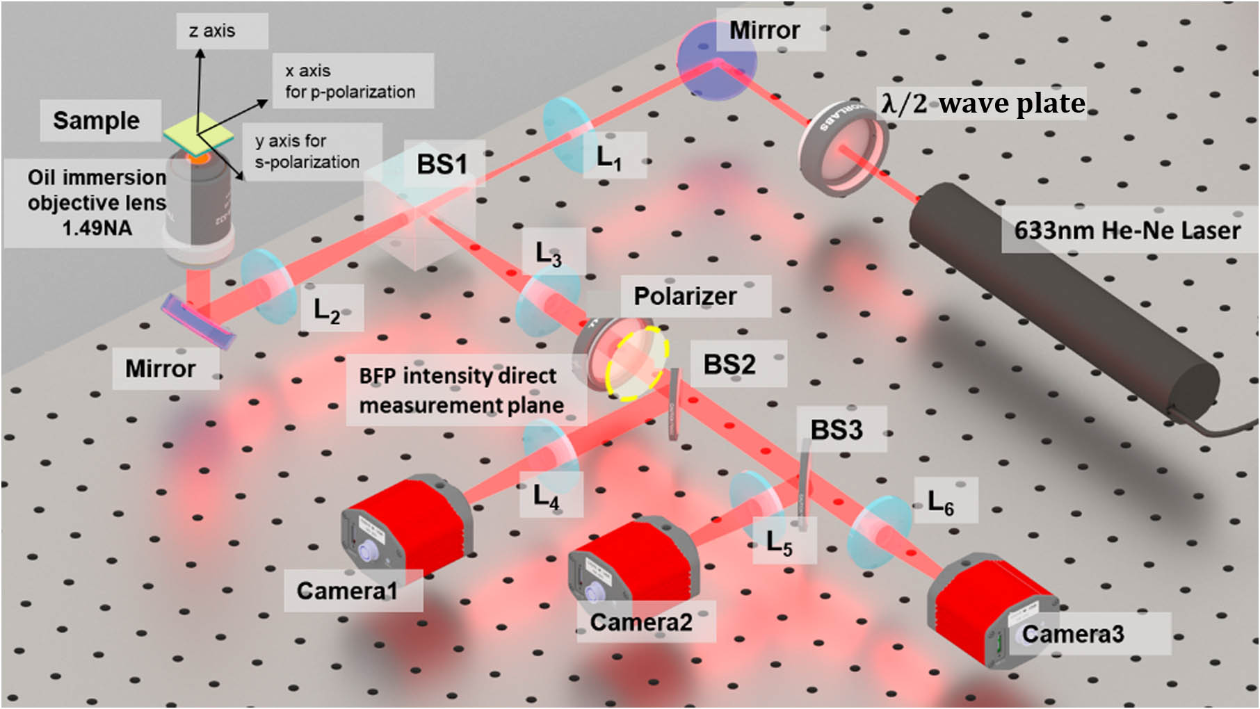
Figure 1.Schematic of the system used to recover the complex field of the BFP, showing three cameras are placed at three corresponding detection arms with various negative defocus positions. One additional arm (the yellow dashed circle plane) was inserted for direct observation of the intensity in the back focal plane. This was not used in any of the reconstructions and simply used for comparison.
The issue of matching the power into multiple planes by cascaded beam splitters is discussed [13]; however, the input data used in our algorithm is close to the Fourier plane of the reconstructed plane (the BFP). Provided sufficiently different defocus distances are used these planes are relatively uncorrelated providing the diversity needed for reliable reconstruction [10], so that the elaborate splitting approach discussed in Ref. [13] is not required.
Sign up for Photonics Research TOC. Get the latest issue of Photonics Research delivered right to you!Sign up now
It is useful to consider the advantages of the three-camera system compared to alternatives. The main advantage of the present system over the system using a single camera as described in Ref. [10] is the far more rapid data acquisition time. With the single-camera system, even when the camera was mounted on a motorized stage the image acquisition took approximately 2 s. In the present three-camera system all the data can be acquired in 42 ms, even with the high dynamic range stitching discussed in Appendix B. This clearly has advantages in monitoring dynamic samples whose properties change with time and also reduces problems with environmental fluctuations. Furthermore, the use of three cameras eliminates the possible problem with registration error of the camera position and reduces the effects of microphonics since all the measurements are taken in parallel rather than serially.
An alternative approach is to use an SLM as the probe. This was used in slightly different context in Ref. [14]. The use of an SLM can remove registration errors and can deliver relatively rapid data acquisition compared to mechanical movement of a camera. The main aim of the present system, however, is for quantitative measurements as discussed in subsequent sections of this paper, and the non-idealities of SLM discourage their use for reliable quantitative measurements. Such deviations from ideality include non-linear phase response, fill factor below 100%, and phase jitter in some commercial SLMs. While these problems are not necessarily insuperable, they introduce unnecessary and avoidable uncertainties into the measurement process.
B. BFP Reconstructions
It is well known that the BFP of a uniform sample maps the reflectivity of the sample with respect to radial position which is proportional to the sine of the incident angle. For linearly polarized light incident on the BFP along one direction (say horizontal) the signal is purely p-polarized (TM), whereas orthogonal to this direction (say vertical) the signal corresponds to pure s polarization (TE). Along other directions the signal results from interference between these components. Separating and extracting these components is necessary to reduce the noise in the measurement. This is discussed in Appendix C.
We carried out two groups of measurements on gold and silver layers, respectively. Five different thicknesses of gold layer were fabricated—35 nm, 41 nm, 47 nm, 53 nm, and 58 nm, respectively—and five different thicknesses of silver layer were also fabricated at 40 nm, 47 nm, 53 nm, 60 nm, and 66 nm. In addition, an 8 nm thick layer of was deposited to avoid the oxidation of silver. These sensors were fabricated using a sputtering machine (Kurt J Lesker, Nano36). A surface profiler was used to calibrate the sputtering machine by measuring the film thickness obtained at a known deposition time. The form of the phase of the reflection coefficient is strongly dependent on the thickness of the metal layer as this strongly controls the loss due to coupling [15]. Tables 1 and 2 show the retrieved phase, retrieved amplitude, and directly measured amplitude of BFPs for gold and silver sensors, respectively. The amplitude is measured by inserting a camera at a plane conjugate to the yellow circle in Fig. 1 for observation and comparison. Retrieved Phase, Retrieved Amplitude, and Measured Amplitude of BFPs for Five Different Thicknesses of Gold Layers Retrieved Phase, Retrieved Amplitude, and Measured Amplitude of BFPs for Five Different Thicknesses of Silver Layers
Figure 2 shows the line traces of the amplitude [Fig. 2(a)] and phase [Fig. 2(b)] of p polarization after noise reduction on gold samples of different thicknesses of 35 nm, 41 nm, 47 nm, 53 nm, and 58 nm, respectively. In Table 1, we can see that apart from the pure p-polarization information, there is also a great deal of information at other azimuthal angles, although along directions other than the horizontal (p polarization) and vertical (s polarization) the two polarization states interfere. We therefore apply a least square algorithm to utilize the available data effectively; this method is described in Appendix C. The same process is used to obtain the line trace of s-polarization information.
![]()
Figure 2.(a) Measured amplitude comparison between various thicknesses of the gold layer along p polarization; (b) retrieved phase transition comparison between different thicknesses of the gold layer along p polarization. The thick layers show the characteristic phase inversion.
Table 2 shows the retrieved phase, retrieved amplitude, and measured amplitude of BFPs of silver layers of different thicknesses of 40 nm, 47 nm, 53 nm, 60 nm, and 66 nm, respectively. Figure 3 shows the line traces of the amplitude [Fig. 3(a)] and phase [Fig. 3(b)] of p polarization after noise reduced on silver samples of different thicknesses of 40 nm, 47 nm, 53 nm, 60 nm, and 66 nm, respectively. By comparing the gold sensor data and silver sensor data, it can be seen that, as expected, the silver layer sensor gives narrower dips and sharper phase transition compared to gold sensors.
![]()
Figure 3.(a) Measured amplitude comparison between various thicknesses of the silver layer along p polarization; (b) recovered phase transition comparison between different thicknesses of the silver layer along p polarization.
3. APPLICATIONS OF THE BFP COMPLEX FIELD
A. Separating the Absorption and Coupling Attenuation Mechanisms
With the reconstructed complex BFP field distributions, we then can separate attenuation due to different mechanisms. When a surface plasmon (SP) is excited, there are two principal loss mechanisms: one is due to the absorption loss and the other arises from coupling loss. Reciprocity indicates that if a wave can be coupled from an external propagating mode it will also leak energy as it propagates. Clearly, surface wave energy lost to absorption is converted to heat, whereas leakage energy is converted to propagating light. Crucial to understanding the measurement of attenuation in a microscope system is to understand that in the confocal system the detected light appears to come from the focus so that, for sufficient defocus, the propagation distance is related to the defocus by (see Fig. 4), where is the defocus and is the angle at which surface plasmons are excited. In a confocal microscope the pinhole will block out light that does not appear to come from the focus, so the confocal system precisely defines the path of the surface waves. This allows the attenuation to be measured. In the microscope system it is straightforward to measure the total attenuation. We only need to examine the decay of the wave as a function of defocus [16]. It is far more challenging to separate the two attenuation mechanisms, and this was addressed in Ref. [11] using an SLM to produce an “artificial” surface wave whose known properties could be used to calibrate the instrument. Let us consider a change in the SP signal modulus with defocus (which as mentioned above can be readily related to the signal change as it propagates along the sample). This can be represented by
![]()
Figure 4.Reradiated leakage propagating light from the surface plasmon.
Therefore, the gradient gives the total attenuation, and the intercept gives the coupling attenuation once the instrumental parameter is available. Separating the two attenuations thus requires the determination of .
The procedures to separate the coupling attenuation and ohmic attenuation are listed as follows.
The attenuation of the surface waves per micrometer propagation distance along the surface is presented in Fig. 7. The blue line is the recovered total attenuation for different metal thicknesses. The red and yellow lines are the coupling loss coefficient and ohmic loss coefficient, respectively. The result agrees with the predicted trends. First, the coupling loss decreases as the thickness of the film increases. Second, the ohmic loss is relatively insensitive to the variation of the thickness. For film thicknesses greater than the penetration depth of SP in the metal (about 30 nm in gold and 26 nm in silver) the absorption loss is almost constant with layer thickness. The results obtained for the absorption loss in the present experiment show far less variability than those obtained by hardware manipulation [11] reinforcing our expectation of the superior robustness and accuracy of the present virtual optics-based measurement. Third, for gold samples, the thickness value where the two attenuation mechanisms intersect is at approximately 46 nm, corresponding to the position where the reflection coefficient approaches zero. For silver samples, the two curves intersect at around 57 nm thickness where the loss due to absorption and coupling loss are equal. The intercept is consistent with the position of the phase inversion of Figs. 2 and 3 where the ohmic loss exceeds the coupling loss. This shows how computational postprocessing of the complex BFP may be used to recover new information; moreover, we reiterate that the noise on the attenuation measurements is considerably smaller than obtained using hardware manipulation of the wavefronts with the SLM.
![]()
Figure 5.(a) Retrieved BFP amplitude distribution for 41 nm thick gold sample; (b) retrieved BFP phase distribution for 41 nm thick gold sample; (c) blue line is the amplitude line trace of p polarization after noise reduction, and black dashed line is the pupil function applied; (d) blue line is the phase line trace of p polarization after noise reduction, and black dashed line is the pupil function applied.
![]()
Figure 6.(a) Normalized experimental
![]()
Figure 7.(a) Attenuation coefficients due to coupling loss and ohmic loss with varying gold thickness; (b) attenuation coefficients due to coupling loss and ohmic loss with varying silver thickness, obtained computationally as opposed to manipulation of the spatial light modulator.
B. Measurement of the Real Part of the Surface Wave
Measurement of the real part of the SP -vector, or the angle at which SPs are excited, is one of the fundamental measurement tasks applied in the sensing of binding and refractive index changes. The advantage, of course, of measurement with an objective lens as opposed to a prism coupler is that the objective lens examines the sample over much finer spatial location providing sensing operations on a microscopic scale.
A direct intensity measurement of the BFP can provide a measure of the -vector by measuring the position of the intensity dips and relating this to the sine of the incident angle for SP excitation. Appendix C shows that different algorithms should be used for separation of the TM and TE components of the reflection coefficient when phase measurement is available compared to the case where only the intensity is measured. The use of the phase signal results in better conditioned reconstruction. Even allowing for the fact that in one case the amplitude of the reflection coefficient is reconstructed and in the other the intensity reflection coefficient is obtained, the overall noise in measuring the dip position is considerably better when the phase measurement is available.
The presence of the BFP phase information also allows virtual optics reconstruction of the -vector. In the previous section we showed that with an appropriate pupil function, , that allows transmission of a wave around the angle for SP excitation and an appropriate defocus the attenuation could be evaluated from the modulus of the where the curve follows the ideal form of Eq. (1). Similarly, if we include the phase variation of the same function, we have
Since the phase of the BFP is available the phase of is readily calculated, which can be equated to in the negative defocus region away from the focus. Measuring the phase gradient over a suitable range of allows the value of to be evaluated and hence the SP wave vector (). It is worth pointing out that the fit to a straight line corresponding to the phase is better than the one used for the attenuation. This is largely because the numerical value of the real part of the -vector is larger than the imaginary part so deviations from linearity are less noticeable.
We therefore have two separate measures of the SP wave vector. The interesting thing is that the noise associated with the values recovered with the two methods is only weakly correlated so the two measures can be combined to improve the overall SNR. The correlation coefficient between these two measurements is only 0.0736. In the present case, the measurement of the obtained from the complex BFP was much better than the dip measurement, so the benefit of combining the measurements was relatively small. These results are presented in Fig. 8. Simulated results which show different noise cases are discussed in Appendix D.
![]()
Figure 8.(a) Dip positions calculated by amplitude; (b) dip positions calculated by
4. CONCLUSION
In this paper we have shown how non-interferometric phase retrieval can be used to perform quantitative measurements in the BFP. The measurements of attenuation and the differences between the gold and silver samples agree well with theory. Phase measurement also has a major advantage for measurement of the SP excitation angle, , as it allows different measurement protocols to be applied to the same data. This allows the better measurement for the particular dataset to be selected. Moreover, the relatively small correlation between different methods allows them to be combined statistically to reduce the noise.
We believe these measures of the phase of the BFP offer new capabilities in objective-based measurements, simplifying the hardware while improving the measurement performance. Further developments will allow the inclusion of reference regions to further enhance measurement precision. Finally, although the present measurements have concentrated on surface wave and SP measurement, the approach described may also be applied to other fields of metrology such as ellipsometry.
Acknowledgment
Acknowledgment. Mengqi Shen led the experimental work and instrument design, analyzed the data, developed the phase retrieval code, and wrote the paper with Michael G. Somekh. Qi Zou carried out experiments and prepared the samples. Xiaoping Jiang carried out the experiments and developed the data acquisition process. Fu Feng analyzed the data and made suggestions to improve the paper. Michael G. Somekh conceived the project, developed the processing algorithms, and wrote the paper with Mengqi Shen. All authors reviewed the paper.
APPENDIX A: RECONSTRUCTION ALGORITHM
The process of phase reconstruction algorithm is shown in Fig.
![]()
Figure 9.Flow chart of three-input phase retrieval algorithm.
Input data: acquire images at three defocus planes and a rough estimate of the window function .
Computational operations on input data are as follows.System.Xml.XmlElementSystem.Xml.XmlElementSystem.Xml.XmlElementSystem.Xml.XmlElementSystem.Xml.XmlElementSystem.Xml.XmlElementSystem.Xml.XmlElementSystem.Xml.XmlElement
APPENDIX B: IMAGE ACQUISITION AND PRE-PROCESSING
The images acquired from the optical system are close to the transform plane; therefore, the pattern will show a sharp peak at the center when close to the focal plane, thus using the available dynamic range of the camera, so that peak values are saturated or small values are swamped by quantization. Using substantial defocus corresponding to a few micrometers at the sample surface greatly relieves this problem; however, to ensure that the low signals are detected while avoiding saturation, multiple exposures are used to increase the dynamic range. This process was automated into the image acquisition process. The process to create high dynamic range (HDR) image is described as follows. Each image is shown in Figs. System.Xml.XmlElementSystem.Xml.XmlElementSystem.Xml.XmlElement
Once
![]()
Figure 10.(a) Normalized intensity comparison between three raw images and the HDR image; (b) shows the coefficients and stitching positions to produce the HDR image; (c) raw image 1 in
![]()
Figure 11.Schematic of BFP for linear polarization.
the coefficients are calculated for each camera, the process is integrated into the image acquisition sequence to generate the HDR images in real time. The total acquisition time including HDR image generation is less than 0.042 s. Normally, because we are using the defocused plane, two images are sufficient to satisfy the dynamic range requirement. Only extreme cases very close to the focus would require three images. To better illustrate the process, below we used three images to show one extreme case at the defocus of .
Figure
APPENDIX C: SEPARATION OF NOISE OF DATA IN BACK FOCAL PLANE
Figure
It can be seen from Fig.
Consider the case where there is no phase information; in this case, we need to work with intensity as given by Eq. (
To get the TM and TE signals, we use a least square approach analogous to that developed by Greivenkamp for phase stepping interferometry [
From these relations standard manipulations lead to a matrix equation:
We take many measurements distributed uniformly between and to form the RHS; this is multiplied by the inverse of the matrix to recover the desired parameters. This results in considerable noise reduction and separates the TM and TE components. This procedure was used in Ref. [
If the phase of the signal is available, we do not need to work with Eq. (
Both formulations allow separation of the TM and TE components and permit noise averaging. The noise reduction is more effective when the phase measurement is available because the condition number of the matrix in Eq. (
APPENDIX D: RELATION BETWEEN NOISE WITH DIFFERENT MEASUREMENT METHODOLOGIES
The fact that we have recovered the phase of the BFP means that we can use different methods to recover the angle for SP excitation . The advantage of this is, of course, if one measurement gives a better result, we can select that methodology. Here, we will also examine situations where we may use both measurements together to get a better result. We will illustrate the ideas in simulation to explain the process and examine the correlations between different methods.
To illustrate the effect of different noise statistics, we consider the following simple model. System.Xml.XmlElementSystem.Xml.XmlElementSystem.Xml.XmlElementSystem.Xml.XmlElementSystem.Xml.XmlElementSystem.Xml.XmlElement
We consider three cases and cutoff frequencies of 125, 35, and 12 noise cycles across the BFP. These illustrative examples are shown in Figs.
![]()
Figure 12.(a) Simulated back focal plane with high-frequency noise case; (b) back focal plane with mid-frequency noise case; (c) back focal plane with low-frequency noise case.
Summarizing the Noise from Different Noise Statistics in the BFPNoise Case Fig. Fig. Fig. Std of Std of Correlation 0.0530 0.0939 Dip signal proportion 0.44 Combined Std
We can see for the high-frequency noise the measurement of the position of the dip gives a far better result compared to the . For the intermediate-frequency noise both methods give comparable noise, and for the low-frequency noise the is clearly superior (this case seems to match our actual experimental results). For the first and last case we could just select the dip position and the , respectively. For the intermediate case we can combine the two measurements using the standard formulation for the sum of correlated variances:
is the total variance; is the fraction of signal 1; is the fraction of signal 2; , are the variances for signals 1 and 2, respectively; and is the correlation between them. To get the correct mean signal it is necessary that .
Table
References
[1] X. Ou, R. Horstmeyer, G. Zheng, C. Yang. High numerical aperture Fourier ptychography: principle, implementation and characterization. Opt. Express, 23, 3472-3491(2015).
[2] J. Sun, C. Zuo, J. Zhang, Y. Fan, Q. Chen. High-speed Fourier ptychographic microscopy based on programmable annular illminations. Sci. Rep., 8, 7669(2018).
[3] H. M. L. Faulkner, J. M. Rodenburg. Movable aperture lensless transmission microscopy: a novel phase retrieval algorithm. Phys. Rev. Lett., 93, 023903(2004).
[4] L. Tian, L. Waller. 3D intensity and phase imaging from light field measurements in an LED array microscope. Optica, 2, 104-111(2015).
[5] A. Ozcan, E. McLeod. Lenless imaging and sensing. Annu. Rev. Biomed. Eng., 18, 77-102(2016).
[6] T. W. K. Chow, B. Zhang, M. G. Somekh. Hilbert transform-based single-shot plasmon microscopy. Opt. Lett., 43, 4453-4456(2018).
[7] S. Pechprasarn, B. Zhang, D. Albutt, J. Zhang, M. Somekh. Ultrastable embedded surface plasmon confocal interferometry. Light Sci. Appl., 3, e187(2014).
[8] C. W. See, M. G. Somekh, R. D. Holmes. Scanning optical microellipsometry for pure surface profiling. Appl. Opt., 35, 6663-6668(1996).
[9] G. D. Feke, D. P. Snow, R. D. Grober, P. J. de Groot, L. Deck. Interferometric back focal plane microellipsometry. Appl. Opt., 37, 1796-1802(1998).
[10] M. Shen, T. W. K. Chow, H. Shen, M. G. Somekh. Virtual optics and sensing of the retrieved complex field in the back focal plane using a constrained defocus algorithm. Opt. Express, 28, 32777-32792(2020).
[11] S. Pechprasarn, T. W. K. Chow, M. G. Somekh. Application of confocal surface wave microscope to self-calibrated attenuation coefficient measurement by Goos-Hanchen phase shift modulation. Sci. Rep., 8, 8547(2018).
[12] L. Allen, M. Oxley. Phase retrieval from series of images obtained by defocus variation. Opt. Commun., 199, 65-75(2001).
[13] A. M. S. Maallo, P. F. Almoro. Power loss due to beam splitter cascade in the simultanous sampling of a volume speckle field for phase retrieval. Proc. SPIE, 7155, 71551J(2008).
[14] P. F. Almoro, Q. D. Pham, D. I. Serrano-Garcia, S. Hasegawa, Y. Hayashi, M. Takeda, T. Yatagai. Enhanced intensity variation for multiple-plane phase retrieval using spatial light modulator as convenient tunable diffuser. Opt. Lett., 41, 2161-2164(2016).
[15] H. Raether. Surface Plasmon on Smooth and Rough Surfaces and on Gratings(1986).
[16] B. Zhang, S. Pechprasarn, M. G. Somekh. Quantitative plasmonic measurements using embedded phase stepping confocal interferometry. Opt. Express, 21, 11523-11535(2013).
[17] J. Greivenkamp. Generalized data reduction for heterodyne interferometry. Opt. Eng., 23, 350-352(1984).
[18] M. Shen, S. Learkthanakhachon, S. Pechprasarn, Y. Zhang, M. G. Somekh. Adjustable microscopic measurement of nanogap waveguide and plasmonic structures. Appl. Opt., 57, 3453-3462(2018).

Set citation alerts for the article
Please enter your email address
© Copyright 2018-2021 | Chinese Laser Press. All Rights Reserved 沪ICP备15018463号-20