Simple and effective method to improve the signal-to-noise ratio of compressive imaging

Yao Zhao; Qian Chen; Guohua Gu; Xiubao Sui

doi:10.3788/COL201715.101101

Abstract

This Letter presents a simple and effective method to improve the signal-to-noise ratio (SNR) of compressing imaging. The main principles of the proposed method are the correlation of the image signals and the randomness of the noise. Multiple low SNR images are reconstructed firstly by the compressed sensing reconstruction algorithm, and then two-dimensional time delay integration technology is adopted to improve the SNR. Results show that the proposed method can improve the SNR performance efficiently and it is easy to apply the algorithm to the real project.

In the past few years, the theory of compressed sensing^[1,2] (CS) has greatly changed the sampling pattern and retrieval scheme. It has been widely used in many areas, such as terahertz (THz) imaging^[3], CS radar^[4], magnetic resonance imaging (MRI)^[5], free-space optical communication^[6], optical fiber communication^[7], and CS imaging^[8]. The advent of the single pixel camera^[9] in 2006 made the compressing imaging become an active research area. Over the next few years, the fast compressive imaging using the scrambled block Hadamard ensemble was proposed, and it can be easily implemented in the optical domain^[10]. Katz et al. proposed a concept termed compressive ghost imaging in 2009^[11]. In 2014, Liutkus et al. proposed a concept named “imaging with nature,” which used the multiply scattering medium as the measurement matrix^[12]. Although compressive imaging breaks the law of Nyquist sampling, the system noise of compressive imaging is inevitable in real applications. For example, for very short exposure imaging, the integration time is very short, and the image signal may be submerged in the noise. Therefore, improving the signal-to-noise ratio (SNR) performance of compressive imaging is of great significance. The way of improving the SNR of compressive imaging can be divided into several categories. For example, the simplest way is to improve the sampling rate. Based on this, we can obtain more measurements. However, a higher sampling rate means that we will deviate from compressive imaging. Another way to improve SNR performance is based on computational constraints in reconstruction phase. Akhlaghi et al.^[13] proposed a compressive correlation imaging method with random illumination, and the authors demonstrated the superior imaging capabilities at low sampling rates and noisy environments. Mao et al. presented a method to improve SNR performance of compressive imaging based on spatial correlation^[14]. The key of the proposed method is second-order correction with the sensing matrix.

In this Letter, we propose a simple and effective method to improve the SNR performance of compressive imaging. The proposed method is mainly based on the two-dimensional time delay integration (2D-TDI) technology, which is usually used in the infrared focal plane array^[15]. 2D means that images are superimposed frame by frame, and TDI is equivalent to increasing the integration time. The mathematical theories of the proposed method are the correlation of the image signals and the non-correlation (randomness) of the noise. Theoretically, the SNR performance of the reconstructed image relies on the number of the superimposed images. The more that images are superimposed, the better the performance of the SNR will be. For example, if the number of images is $m$ , then the SNR can be improved by $\sqrt{m}$ times than before. The detailed analysis about the proposed method will be illustrated in three parts as follows. First, the system architecture of the proposed method is introduced, and then the framework of the compressive imaging under strong noise is analyzed. Finally, we explain how to improve the SNR performance by 2D-TDI, and the corresponding results are discussed.

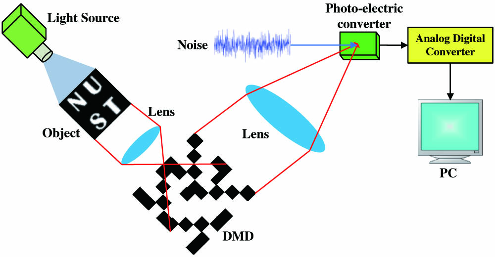
Figure 1 shows the schematic of the system setup. The system is basically an optical computer [comprising a light source, the object to be imaged, a digital micro-mirror device (DMD), two lenses, a photo-electric converter, an analog-to-digital converter (ADC), and a computer], which computes the random linear measurements of the object under view.

Sign up for Chinese Optics Letters TOC. Get the latest issue of Chinese Optics Letters delivered right to you！Sign up now

Figure 1.Schematic of the setup.

The object is focused by a biconvex lens onto the DMD, which consists an array of $N$ tiny micro-mirrors. The cell size of the DMD is 7.6 μm, and the active area is 6.8 μm. During the compressive imaging processing, the DMD will be changed $M$ times to obtain $M$ measurements. From the above setup, we can see that each measurement contains the complete information of the object. Then, the compressive imaging can be represented as $y = Φ_{M N} x,$ (1)where $x$ is an $N \times 1$ vector that represents the object signal, and $N$ is the number of the pixels. $y$ is the compressed image signal, which also can be represented as a vector $M \times 1$ . $x = {x_{1}, x_{2}, x_{3} \dots x_{N}}^{T}$ , and $y = {y_{1}, y_{2}, y_{3} \dots y_{M}}^{T}$ . In the framework of compressive imaging, $M < N$ and $M / N$ represents the sampling rate. $Φ_{M N}$ is the measurement matrix, which can be implemented by the DMD. In normal conditions, $Φ_{M N}$ is set as a random Gaussian matrix. The recovery $x$ from $y$ is usually called sparse reconstruction when the object is sparse. But, if the object is not sparse, the imaging model can be modified as $y = Φ_{M N} x = Φ_{M N} ψ α,$ (2)where $α$ is the sparse coefficient, and $ψ$ is a sparse basis. $ψ$ is always set as the Fourier basis or wavelet basis. Reconstruction algorithms, such as orthogonal matching pursuit (OMP)^[16] or TV minimization by augmented Lagrangian and alternating direction algorithm (TVAL3)^[17], are two popular methods to reconstruct the original signal from compressed sampling points. Figure 2 shows the reconstruction results of compressive imaging under a noise-free environment. Figure 2(a) is an original image with the spatial resolution of $96 \times 96$ . Figure 2(b) is the reconstructed image under a noise-free condition. The reconstruction algorithm is chosen as TVAL3 and the sampling rate is set as 0.1. We can see from visualization that in noise-free environment and TVAL3 algorithm can reconstruct the image with high SNR.

Figure 2.Reconstruction results of compressive imaging under a noise-free environment. (a) Original image with the spatial resolution of $96 \times 96$ ; (b) the reconstructed image by TVAL3 under a noise-free condition.

In order to evaluate the reconstruction performance objectively, the peak SNR (PSNR) is introduced, and it is defined as $PSNR (dB) = 10 \times \log_{10} \frac{255^{2}}{MSE} .$ (3)

The mean square error (MSE) is shown as $MSE = \frac{1}{M \times N} \sum_{i = 1}^{M} \sum_{j = 1}^{N} e^{2} (i, j),$ (4)where $M$ and $N$ are the column and row numbers of an image, respectively, and $e (i, j)$ is the difference between the original image and reconstructed image at a pixel location. The MSE between the reconstructed image [Fig. 2(b)] and the original image [Fig. 2(a)] is 80.3971, and the PSNR of the reconstructed image is 29.0784 dB.

However, in the real application of compressive imaging, noise is inevitable, and sometimes signals will be covered by strong noise. Figure 3 shows the reconstruction results of compressive imaging in different noise environments, and the reconstruction algorithm is still chosen to be TVAL3. The spatial resolution of the images is still $96 \times 96$ . Sampling rates are all set as 0.6. Figure 3(a) is the reconstructed image in 45 dBW (dBW represents the power of the noise) Gaussian noise environment; we can see that there is small amount of random point noise in the reconstructed image, but the performance of the reconstructed image is still satisfied. Figures 3(b)–3(d) are reconstructed images in 55, 60, and 65 dBW noise environments, respectively. As we can see, that while the noise is increasing, signals are gradually covered by noise. The PSNRs of the following reconstructed images are 23.6373, 13.4012, 10.6573, and 9.4279 dB, respectively.

Figure 3.Reconstruction results of the compressive imaging in different noise environments.

We then analyze the mathematical framework of the compressive imaging in a noisy condition (assume the object is sparse). The compressive imaging in a noisy environment can be represented as $y^{'} = Φ_{M N} x + n,$ (5)where $y^{'}$ is the compressed signal in noisy condition, and $n$ represents random noise. Further, Eq. (5) can be represented as another form, $y^{'} = y + n,$ (6)where $y$ is the compressed image signal in the noise-free condition. This suggests that the compressed signal in the noisy condition can be considered as the sum of image signal and noise. The reconstruction of compressive imaging is to obtain image signal $x^{'}$ (with noise) from compressed signal $y^{'}$ ; $y^{'} = y + n = Φ_{M N} x^{'} .$ (7)

The solution of the Eq. (7) is to solve the optimization problem $\min λ {‖ x_{0}^{'} ‖}_{1} + \frac{1}{2} {‖ y^{'} - Φ_{M N} x_{0}^{'} ‖}_{2}^{2} .$ (8)

Here, $x_{0}^{'}$ is the solution of the Eq. (7), and it is equivalent to image $x^{'}$ . $λ$ balances the sparsity of the solution and the fidelity of the approximation to $y^{'}$ . We let $x^{'} = x + g$ , thus, Eq. (7) can be further expressed as $y + n = Φ_{M N} (x + g) = Φ_{M N} x + Φ_{M N} g .$ (9)

Thus, the solution of the Eq. (9) can be regarded as the sum of two optimization problems, which can be written as $\min λ_{1} {‖ x_{0} ‖}_{1} + \frac{1}{2} {‖ y - Φ_{M N} x_{0} ‖}_{2}^{2},$ (10) $\min λ_{2} {‖ g_{0} ‖}_{1} + \frac{1}{2} {‖ n - Φ_{M N} g_{0} ‖}_{2}^{2} .$ (11)

Therefore, the reconstructed signal $x^{'}$ can be thought as the sum of $x_{0}$ and $g_{0}$ . $x_{0}$ represents the original image signal, and $g_{0}$ represents the noise. Note, $g_{0}$ is not equal to $n$ , but they all have the same characteristic of random distribution. From the above equations, we can draw a conclusion that under the noisy condition, the reconstructed signal can still be regarded as the sum of image signal and noise, and even in a strong noise environment, the image signal is still retained in the reconstructed signal.

Based on the above conclusion, we can use the correlation of the image signal and the randomness (non-correlation) of the noise to improve the performance of SNR. Here, we adopt 2D-TDI technology to improve the SNR of the compressive imaging. The principles of improving the SNR by 2D-TDI are the correlation of the image signals and the non-correlation of the noise. Assume the object in Fig. 1 is static or moving slowly, and there are $m$ frame reconstructed images to be used in the 2D-TDI method. As we all know, power is proportional to the square of the voltage. Thus, the power of the reconstructed image signal after the 2D-TDI algorithm can be expressed as $P_{S} = {(\sum_{i = 1}^{m} V_{s i})}^{2} = \sum_{i = 1}^{m} V_{s i}^{2} + 2 \sum_{i = 1}^{m} \sum_{j = 1}^{i - 1} C_{i, j} V_{s i} V_{s j},$ (12)where $V_{s i}$ and $V_{s j}$ are the $i th$ and $j th$ reconstructed image signals, and $C_{i, j}$ is the correlation coefficient between $V_{s i}$ and $V_{s j}$ , $0 \leq C_{i, j} \leq 1$ . Similarly, the power of noise can also be expressed as $P_{N} = {(\sum_{i = 1}^{m} V_{N i})}^{2} = \sum_{i = 1}^{m} V_{N i}^{2} + 2 \sum_{i = 1}^{m} \sum_{j = 1}^{i - 1} C_{i, j}^{N} V_{N i} V_{N j},$ (13)where $V_{N i}$ and $V_{N j}$ are the $i th$ and $j th$ noise signals, and $C_{i, j}^{N}$ is the correlation coefficient between $V_{N i}$ and $V_{N j}$ . As we all know, random noise has the characteristics of non-correlation. Thus, theoretically, $C_{i, j}^{N} = 0$ . Then, Eq. (13) can be expressed as $P_{N} = {(\sum_{i = 1}^{m} V_{N i})}^{2} = \sum_{i = 1}^{m} V_{N i}^{2} = m V_{N}^{2},$ (14)where $V_{N}$ is the equivalent noise. Due to the object being static or moving slowly, the correlation between each image signal is very high. So, $C_{i, j}$ approximately equals one. Thus, Eq. (12) can be further expressed as $P_{S} = {(\sum_{i = 1}^{m} V_{s i})}^{2} = \sum_{i = 1}^{m} V_{S}^{2} + 2 C_{m}^{2} V_{S}^{2} = m^{2} V_{S}^{2},$ (15)where $V_{s i}$ is the image signal in the $i th$ frame, and $V_{S}$ represents the equivalent image signal. Thus, the SNR of power is ${SNR}_{(power)} = \frac{P_{S}}{P_{N}} = \frac{m^{2} V_{S}^{2}}{m V_{N}^{2}} .$ (16)

We note that the original power SNR is ${SNR}_{0}$ , and the ${SNR}_{0}$ can be expressed as ${SNR}_{0} = \frac{V_{S}^{2}}{V_{N}^{2}} .$ (17)

Thus, we have the conclusion that ${SNR}_{(power)} = m \cdot {SNR}_{0 (power)} .$ (18)

From Eq. (18), we can see that the power SNR is $m$ times more than before. Due to the fact that power is proportional to the square of the voltage, thus, the SNR of the image is $\sqrt{m}$ times more than before, as shown in Eq. (19), where $m$ is the number of frames; $SNR = \sqrt{m} \cdot {SNR}_{0} .$ (19)

We then evaluate the performance of the proposed method by numerical simulations. PSNR (dB) is adopted, and it is already introduced above. Figure 4(a) shows the reconstructed image under 55 dBW Gaussian noise. The spatial resolution of the images in Fig. 4 are $96 \times 96$ . Figures 4(b)–(d) are reconstructed images by the proposed method with $m = 5$ , 10, and 15, respectively. We can see from Fig. 4 that with the increasing of $m$ , the SNR performance is gradually improving.

Figure 4.(a) Reconstructed image under 55 dBW Gaussian noise; reconstructed images by the proposed method with $m = (b) 5$ , (c) 10, and (d) 15.

Then, we compute the PSNRs of the reconstructed images under different numbers of $m$ , and the Gaussian noise is also set as 55 dBW. Table 1 and Fig. (5) show the relationship between PSNRs and $m$ . We can see that PSNRs increase as $m$ increases. But, the relationship is not consistent with Eq. (19). This is because the correlation coefficients are not actually zero or one.

Number of m	1	5	10	15	20
PSNR (dB)	14.005	17.841	19.792	20.676	21.612

Table 1. Relationship between PSNRs and m

View all Tables

Figure 5.Relationship between PSNRs and $m$ .

Next, we consider a situation of a strong noise condition. The image signal is covered by noise, as shown in Fig. 6(a). The Gaussian noise is 65 dBW. We then verify the performance of the proposed method, and the letters “NUST” are still chosen as the test image.

From Fig. 6, we can see that even in a strong noise condition, the proposed algorithm is still able to improve the SNR.

Figure 6.(a) Reconstructed image under 65 dBW Gaussian noise; (b) reconstructed image by the proposed method with $m = 30$ (65 dBW noise).

In conclusion, we propose a simple and effective method to improve the SNR of compressive imaging. First, we illustrate the principles of compressive imaging, and then the reconstruction model under a noisy condition is introduced. Finally, the way of improving SNR based on the correlation of the image signals and randomness of noise are analyzed, and the performance is also verified.

References

[1] D. L. Donoho. IEEE Trans. Inform. Theory, 52, 1289(2006).

[2] E. J. Candès, M. B. Wakin. IEEE Signal Process. Mag., 25, 21(2008).

[3] Y. Li, Q. Li, J. Hu, Y. Zhao. Chin. Opt. Lett, 13, S11101(2015).

[4] S. Bhattacharya, T. Blumensath, B. Mulgrew, M. Davies. Proceeding of 14th Workshop on Statistical Signal Processing, 448(2007).

[5] M. Lusting, D. Donoho, J. Santos, J. Pauly. IEEE Signal Process. Mag., 25, 72(2008).

[6] T. Mao, Q. Chen, W. He, Y. Zou, H. Dai, G. Gu. Chin. Opt. Lett., 14, 110607(2016).

[7] B. Hui, X. Tang, N. Gao, W. Zhang, X. Zhang. Chin. Opt. Lett., 14, 110602(2016).

[8] P. Nagesh, B. Li. Proceeding of Acoustics, Speech and Signal Processing, 1261(2009).

[9] M. F. Duarte, M. A. Davenport, D. Takhar, J. N. Laska, T. Sun, K. F. Kelly, R. G. Baraniukm. IEEE Signal Process. Mag., 25, 83(2008).

[10] L. Gan, T. T. Do, D. Tran. Proceeding of European Signal Processing(2008).

[11] O. Katz, Y. Bromberg, Y. Silberberg. Appl. Phys. Lett., 95, 131110(2009).

[12] A. Liutkus, D. Martina, S. Popoff, G. Chardon, O. Katz, G. Lerosey, S. Gigan, L. Daudet, L. Carron. Sci. Rep., 4, 5552(2014).

[13] M. I. Akhlaghi, A. Dogariu. Opt. Lett., 40, 4464(2015).

[14] T. Mao, Q. Chen, W. He, Y. Zou, H. Dai, G. Gu. Opt. Rev., 23, 571(2016).

[15] X. Sui, Q. Chen, L. Bai, G. Gu. Infrared Laser Eng., 39, 993(2010).

[16] J. A. Tropp, A. C. Gilbert. IEEE Trans. Inform. Theory, 53, 4655(2007).

[17] C. Li. An efficient algorithm for total variation regularization with application to the single pixel camera and compressive sensing(2009).