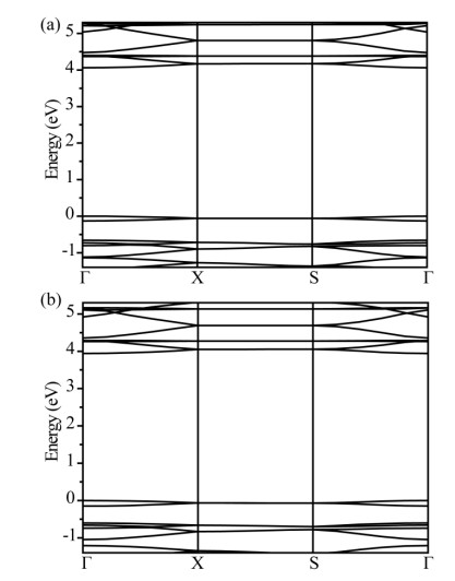
Fig. 1. GW band structure of the monolayer sp²c-COF in the ground-state geometry optimized by DFT (a) and that in the excited-state geometry optimized by the constrained DFT (b). In the constrained DFT, populations of the highest occupied molecular orbital (HOMO) and the lowest unoccupied molecular orbitals are both set to one. The GW band gap in (b) is smaller than that in (a) by 0.12 eV.

Fig. 1. (a, b) Structure of sp\begin{document}$ ^2 $\end{document}c-COF-2. (c, d) Structure of sp\begin{document}$ ^2 $\end{document}c-COF. Rectangles in (b, d) represent the primitive cell of respective COF.

Fig. 2. (a) Crystal structure of sp\begin{document}$ ^2 $\end{document}c-COF. (b) and (c) are the side view and the top view of sp\begin{document}$ ^2 $\end{document}c-COF respectively.

Fig. 2. Optical absorption spectrum of the monolayer sp²c-COF in the ground-state geometry optimized by DFT (black curve) and that in the excited-state geometry optimized by the constrained DFT (red curve). The exciton momentum q→0. The direction of exciton momentum is parallel to the lattice vector \begin{document}$\vec c$\end{document}. Absorption peaks in the excited-state geometry redshift by 0.08 eV compared to those in the ground-state geometry.

Fig. 3. Band structures of sp\begin{document}$ ^2 $\end{document}c-COF-2. (a, b) Bulk sp\begin{document}$ ^2 $\end{document}c-COF-2. (c) First Brillouine zone of bulk sp\begin{document}$ ^2 $\end{document}c-COF-2, (d, e) monolayer sp\begin{document}$ ^2 $\end{document}c-COF-2. (a, d) are calculated by DFT-LDA, while (b, e) are calculated by GW.

Fig. 3. LDA band structure of the AA-stacked bulk sp²c-COF in the ground-state geometry optimized by DFT (a) and that in the excited-state geometry optimized by the constrained DFT (b). The band gap in (b) is smaller than that in (a) by 0.09 eV.

Fig. 4. Charge density distributions (purple and yellow isosurfaces) of four bands in sp\begin{document}$ ^2 $\end{document}c-COF-2.

Fig. 5. Optical absorption spectra of sp\begin{document}$ ^2 $\end{document}c-COF-2 with the exciton momentum \begin{document}$ q $\end{document}\begin{document}$ \rightarrow $\end{document}0. (a, b, c) Spectra of bulk sp\begin{document}$ ^2 $\end{document}c-COF-2 with the direction of exciton momentum parallel to lattice vectors \begin{document}$ \vec a $\end{document}, \begin{document}$ \vec b $\end{document}, and \begin{document}$ \vec c $\end{document} respectively. (d) Spectrum of monolayer sp\begin{document}$ ^2 $\end{document}c-COF-2. Black and red curves represent the spectra which are broadened artificially by 0.1 eV and 0.3 eV respectively. T\begin{document}$ _1 $\end{document} represents position of the lowest triplet exciton. S\begin{document}$ _1 $\end{document} and S\begin{document}$ _2 $\end{document} represent positions of the lowest and the second lowest singlet excitons. The blue dashed curves show the experimental absorption spectra from Ref.[20].

Fig. 6. Main compositions of the lowest singlet exciton of bulk sp\begin{document}$ ^2 $\end{document}c-COF-2 in the first Brillouine zone depicted in (a), a 3\begin{document}$ \times $\end{document}3\begin{document}$ \times $\end{document}15 \begin{document}$ k $\end{document}-point grid is used to represent excitonic wave functions in our BSE calculations. (b), (c), and (d) illustrate the contributions from \begin{document}$ k $\end{document} = (\begin{document}$ k_x $\end{document}, \begin{document}$ k_y $\end{document}, \begin{document}$ k_z $\end{document}) points distributed on the planes colored in blue (\begin{document}$ k_z $\end{document} = 0), red (\begin{document}$ k_z $\end{document} = 1/15\begin{document}$ |Z| $\end{document}), and green (\begin{document}$ k_z $\end{document} = 2/15\begin{document}$ |Z| $\end{document}) shown in (a), respectively.

Fig. 7. Real-space distributions of photoelectrons (red isosurfaces) for excitons in bulk sp\begin{document}$ ^2 $\end{document}c-COF-2. (a, b) The lowest exciton at 2.10 eV, and (c, d) the exciton at 2.67 eV. (a, c) Top views and (b, d) side views. The hole is fixed at atoms enclosed inside the rectangle depicted in (a, c).

Fig. 8. Theoretical optical absorption spectra of bulk sp\begin{document}$ ^2 $\end{document}c-COF-2 for excitons with finite momenta (in Å\begin{document}$ ^{-1} $\end{document}). Directions of the exciton momenta are parallel to the \begin{document}$ \Gamma $\end{document}-\begin{document}$ Z $\end{document} direction in the first Brillouin zone. \begin{document}$ q $\end{document} = 0.840 corresponds to the \begin{document}$ Z $\end{document} point. Right panels are enlarged views of the corresponding left ones. Vertical lines in the left panels mark energies of the lowest five excited states.

Fig. 9. Distributions of the photoelectron and hole in the first Brillouine zone for the exciton with the momentum \begin{document}$ q $\end{document} = 0.336 Å\begin{document}$ ^{-1} $\end{document} in bulk sp\begin{document}$ ^2 $\end{document}c-COF-2. A 3\begin{document}$ \times $\end{document}3\begin{document}$ \times $\end{document}15 \begin{document}$ k $\end{document}-point grid is used to represent excitonic wave functions in our BSE calculations. (a) Distribution of hole for the lowest exciton. (b) Distribution of photoelectron for the second lowest exciton. Each red horizontal column illustrates the sum of contributions from the \begin{document}$ k $\end{document} points distributed on the corresponding blue plane in the first Brillouine zone.

Fig. 10. Band structures of bulk sp\begin{document}$ ^2 $\end{document}c-COF. (a, b) AA-stacked sp\begin{document}$ ^2 $\end{document}c-COF, (c) AB-stacked sp\begin{document}$ ^2 $\end{document}c-COF. (a, c) are calculated by DFT-LDA, while (b) is calculated by GW. (d) Top view of AB-stacked sp\begin{document}$ ^2 $\end{document}c-COF where the brown and the blue atoms belong to different layers.

Fig. 11. Optical absorption spectrum of AA-stacked sp\begin{document}$ ^2 $\end{document}c-COF with the exciton momentum \begin{document}$ q $\end{document}\begin{document}$ \rightarrow $\end{document}0 and the direction of exciton momentum parallel to the lattice vector \begin{document}$ \vec c $\end{document}. S\begin{document}$ _1 $\end{document} represents position of the lowest singlet exciton. The blue dashed curve shows the experimental absorption spectrum from Ref.[20].

Table 1. Lattice parameters of sp$ ^2 $c-COF and sp$ ^2 $c-COF-2 from experiments and theoretical calculations.