LS-SVM-based surface roughness prediction model for a reflective fiber optic sensor

Li Fu; Jun Luo; Weimin Chen; Xueming Liu; Dong Zhou; Zhongling Zhang; Sheng Li

doi:10.3788/COL201715.091201

Abstract

Reflective fiber optic sensors have advantages for surface roughness measurements of some special workpieces, but their measuring precision and efficiency need to be improved further. A least-squares support vector machine (LS-SVM)-based surface roughness prediction model is proposed to estimate the surface roughness, Ra, and the coupled simulated annealing (CSA) and standard simplex (SS) methods are combined for the parameter optimization of the mode. Experiments are conducted to test the performance of the proposed model, and the results show that the range of average relative errors is

4.232 % - 2.5709 %

. In comparison with the existing models, the LS-SVM-based model has the best performance in prediction precision, stability, and timesaving.

Quantitative estimations of surface roughness can be realized by different methods, such as a stylus^[1], image-based spectral correlation^[2], speckle^[3], and optical scattering^[4–8]. Since the optical scattering method can make use of small and flexible fiber optic sensors^[4,8], it is more suitable for internal surface roughness measurements of small workpieces or complex structures. Based on the Beckmann scattering model^[9], the surface roughness can directly be calculated by the scattering-to-specular or specula-to-total light intensity ratio. Also, the model can be used as a fitting model for precalibration^[10,11].

The Beckmann scattering model is established on the scalar scattering theory, so it cannot accurately characterize the nonlinear relationship between the light intensity ratio and surface roughness. Worse, measuring uncertainty may further amplify the final error. For example, Refs. [10,11] provide a maximum relative error larger than 10%. To better solve the nonlinear problem, some surface roughness prediction models are proposed, such as the back-propagation neural network (BPNN) model^[12,13], and the support vector machine (SVM) model^[14]. However, the BPNN has some disadvantages, such as getting stuck easily in local minima and a long training time, as well as especially poor generalization when solving practical problems with few samples^[15,16]. The SVM using gridregression.py for parameter optimization in Ref. [14] requires a long computation time. The least-squares (LS) SVM^[17] is a reformulation of the standard SVM^[18], which lead to solving linear Karus–Kuhn–Trucker (KKT) systems. In contrast to BPNN and SVM, the LS-SVM model requires shorter calculation times and has a more powerful computational ability in solving the nonlinear and small sample problems. In this Letter, an LS-SVM-based surface roughness prediction model is proposed by combining the coupled simulated annealing (CSA) and standard simplex (SS) methods. To the best of our knowledge, it has the best prediction performance among the reported models.

When a surface is irradiated by a laser beam, the incident light is scattered. Assuming that the surface absorption of the light is negligible, some of the scattered light, following the law of geometrical optics, reflects in the specular direction, and the other portion is scattered into space in all directions. According to Beckmann’s theory, if the incident light is vertical to the surface, the relationship between the relative value of the scattered light intensity $I$ , the scattering angle $θ_{2}$ , and the surface profile’s RMS deviation $R_{q}$ can be described as^[19] $I = {{{\frac{\sin [(2 π L / λ) \sin θ_{2}]}{(2 π L / λ) \sin θ_{2}}}^{2}} + \frac{T \sqrt{π}}{2 L} \sum_{m = 1}^{\infty} \frac{{[{(2 π R_{q} / λ) (1 + \cos θ_{2})]}^{2}}^{m}}{m! \sqrt{m}} \times \exp {- \frac{{[(2 π T / λ) \sin θ_{2}]}^{2}}{4 m}}} \times \exp {- {[(2 π R_{q} / λ) (1 + \cos θ_{2})]}^{2}},$ (1)where $λ$ is the wavelength of the incident light, $2 L$ is the surface length, and $T$ is the correlation length of the surface. This relation can also be described as $I = \frac{I_{o}}{I_{i}},$ (2)where $I_{o}$ is the scattering light intensity, and $I_{i}$ is the reflected light intensity in the specular direction, as the light is incident on an ideal flat surface. Since it is difficult to obtain an ideal flat surface, usually, $I_{i}$ is replaced by the incident light intensity.

Sign up for Chinese Optics Letters TOC. Get the latest issue of Chinese Optics Letters delivered right to you！Sign up now

For the same surface, the relationship between $R_{q}$ and $R_{a}$ can be approximated as a linear function, and $L$ and $T$ can also be treated as constants. Additionally, for the same incident light condition, $λ$ is a constant. Since the light intensity is the light power of the per unit area, the above derivation shows that the relative light power is a unary nonlinear function of $R_{a}$ , and Eq. (1) can be simplified into $\frac{P_{o}}{P_{i}} = f (R_{a}),$ (3)where $P_{o}$ is the power of the scattered light, and $P_{i}$ is the power of the incident light.

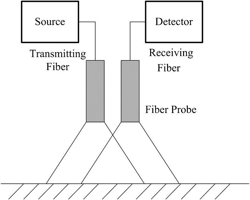
The schematic in Fig. 1 shows the principle of measuring the surface roughness through the reflective fiber optic sensors. When the incident laser light arrives at the measured surface through the transmitting fiber, the incident light is scattered. This surface-scattering light enters the receiving fiber, and the light power is measured by a detector^[20]. Although the receiving fiber may not receive all of the scattered light, the above analysis indicates that under certain measurement conditions and within the same receiving angular range, the ratio between the received light power and the incident light power is related to $R_{a}$ . Therefore, the surface roughness $R_{a}$ is represented by the ratio.

Figure 1.Schematic diagram of surface roughness measurement using reflective fiber optic sensors.

It is assumed that $x_{i}$ is the aforesaid power ratio for the $i$ th test point on the measured surface, and $y_{i}$ is the roughness value of the point, where $i = 1, 2, \dots, N$ . The combination of ( $x_{i}$ , $y_{i}$ ) provides the training sample set for the LS-SVM model. The task of the LS-SVM-based roughness prediction model is to determine the nonlinear relationship between $y_{i}$ and $x_{i}$ : $y_{i} = f (x_{i}) .$ (4)

Based on the theory of SVM, the following model is constructed by using the nonlinear mapping function $ϕ (x)$ , which maps the input space to a higher dimensional space, $f (x) = ω^{T} ϕ (x) + b,$ (5)where $b$ is offset, and $ω$ is weight vector of the same dimensions as the feature space.

The values of $ω$ and $b$ can be obtained via minimizing the following regularized cost functions: $\min J (ω, e) = \frac{1}{2} ω^{T} ω + \frac{γ}{2} \sum_{i = 1}^{N} e_{i}^{2},$ (6) $subject to y_{i} = ω^{T} ϕ (x_{i}) + b + e_{i},$ (7)where $γ$ is a regularization parameter, $e_{i}$ is the e-insensitive error, and $b$ is a constant bias. The above constrained optimization problem can be converted into an unconstrained optimization problem by constructing the Lagrange function as $L (ω, b, e, α) = J (ω, e) - \sum_{i = 1}^{N} α_{i} [ω^{T} ϕ (x_{i}) + b + e_{i} - y_{i}],$ (8)where $α_{i}$ is the Lagrange multiplier. The conditions for optimality are given by partially differentiating with respect to each variable. Eliminating $ω$ and $e$ , the KKT system is obtained as $[\begin{matrix} 0 & 1_{l}^{T} \\ 1_{l} & Ω + γ^{- 1} I \end{matrix}] [\begin{matrix} b \\ a \end{matrix}] = [\begin{matrix} 0 \\ Y \end{matrix}],$ (9)where $1_{l} = {[\begin{matrix} 1 & 1 & \dots & 1 \end{matrix}]}^{T}$ , $a = {[\begin{matrix} a_{1} & a_{2} & \dots & a_{N} \end{matrix}]}^{T}$ , $Y = (y_{1}, y_{1}, \dots, y_{N})$ . $Ω$ is the kernel function, defined as $Ω_{i, j} = ϕ {(x_{i})}^{T} \cdot ϕ (x_{j}) = K (x_{i}, x_{j}) .$ (10)

Here, $j = 1, 2, \dots, N$ .

When $a$ and $b$ are resolved using Eq. (9), the LS-SVM-based surface roughness prediction model can be obtained as $f (x) = \sum_{i = 1}^{N} a_{i} K (x, x_{i}) + b,$ (11)and after the model is trained with a training sample set, the surface roughness can be calculated by the received-to-incident light power ratio $x$ in the testing sample set and Eq. (11).

The radial basis function (RBF) [Eq. (12)] is selected as a kernel function due to its high regression precision, $K (x, x_{i}) = \exp [(- {‖ x - x_{i} ‖}^{2}) / σ^{2}],$ (12)where $σ^{2}$ is the kernel width of the RBF.

Because the tuning parameters, $γ$ and $σ^{2}$ , influence the performance of the LS-SVM model, their values should be optimized in advance. The CSA algorithm is introduced here to globally search a relatively good initial value. Then, the SS algorithm is used for a finer search in the neighborhood of the initial value^[21].

In detail, the steps of the surface roughness prediction are as follows: (1)Acquiring sample data, which include the training sample set and testing sample set described above.(2)Setting the tuning parameters, $γ$ and $σ^{2}$ .(3)Establishment of the surface roughness prediction model. The model parameters $a$ and $b$ in Eq. (9) are solved by identifying the training sample set and then substituted into Eq. (11) to obtain the model.(4)Calculation of the surface roughness and prediction errors. The input values of the test sample set are substituted into the prediction model to obtain the prediction of the surface roughness, which is then compared with the expected result to calculate the prediction error.

In order to acquire the sample data of the LS-SVM mode, the surface roughness measuring system is designed as shown in Fig. 2. The fiber optic probe is fixed on an adjustable XYZ displacement platform and perpendicular to the surface of the specimen. An amplified spontaneous emission (ASE) light source^[22,23] with a 1550 nm working wavelength is chosen as the light source for its good output power stability. The optical power meter detecting the light power has $\pm 0.02 dB$ linearity and a 0.01 dB display resolution. The coaxial fiber bundle structure is chosen because it has the advantage of stability of measurement compared with the noncoaxial fiber bundle when the working distance between the probe and the measured surface is the peak interval of the light intensity modulation curve. Figure 3 displays the end-face structure of the fiber optic probe. The central fiber is the transmitting fiber, and the six fibers surrounding it are receivers. Both the transmitting and receiving fibers are multimode fibers with a 105 μm core diameter and a 0.22 numerical aperture.

Figure 2.Measuring system.

Figure 3.End-face structure of fiber optic probe.

Standard specimens with nonplanar rough surfaces are used as measured objects, which are machined by internal grinding and circular grinding with four levels. The light intensity modulation curve of the fiber bundle shows that the reflected light intensity is the most sensitive to the change of the surface roughness at the peak point^[10,24]; therefore, the abscissa of the point obtained by repeated tests is used as the working distance between the probe and the measured surface, which is 0.87 and 0.91 mm for the internal and circular grinding specimens, respectively.

In the experiment, 40 different points for each specimen are measured in the $X - Y$ plane. Half of the measured points are used as the training sample set.

To verify the advantages of the LS-SVM model, BPNN and SVM are used for comparison. The three modes are implemented using the LS-SVMlab1.8 toolkit (http://www.Esat.kuleuven.be/Sista/lssvmlab/), the LIBSVM toolbox (https://www.csie.NTU.edu.tw/~cjlin/libsvm/), and the BPNN toolbox of MATLAB software, respectively. All calculations were performed using MATLAB 7.8.0, which are done on an Intel core (TM) M-5Y10c 0.80 GHz with 8GB RAM.

A three-layer BPNN model is used for its good performance in predicting nonlinear relationships^[25]. Based on the Kolmogorov theorem, the calculated numbers of the hidden layer neurons are 2 to 11. The chosen number is 10 according to the optimal result from the simulations of the total of 10 different numbers of hidden layer neurons. The input function, training function, and output function are logsig, traingdx, and purelin, respectively. The number of iterations is set at 200.

For the LS-SVM model, the optimized parameter values for $γ$ / $σ^{2}$ are 188585.755/0.0181 and 60.659/0.0419 for the internal and circular grinding specimens, respectively. For a fair comparison, the kernel function for the SVM model is the same as that of the LS-SVM model. As described in Ref. [15], the optimal values for the unspecified parameters (the optimal penalty parameter $c$ , the number of attributes $g$ , and the epsilon in the loss function $p$ ) are searched automatically with gridregression.py. They are 64, 32, 0.000977 and 1024, 32, 0.0313 for the internal and circular grinding specimens, respectively.

The prediction accuracy and stability of three models are quantitatively evaluated by the mean surface roughness ( ${MR}_{a}$ ), mean relative error ( $MRE$ ), and standard deviation ( $SD$ ). They are defined as follows: ${MR}_{a} = \frac{1}{N} \sum_{i = 1}^{N} R_{ai},$ (13) $MRE = (\frac{1}{N} \sum_{i = 1}^{N} \frac{R_{ai} - R_{aN}}{R_{aN}}) \times 100 %,$ (14) $SD = \sqrt{\frac{1}{N - 1} \sum_{i = 1}^{N} {(R_{ai} - \bar{R_{a}})}^{2}},$ (15)where $R_{ai}$ is the predicated roughness value for the $i$ th test point, $N$ is the number of test samples, $R_{aN}$ is the nominal roughness value of the surface roughness specimen, and ${\bar{R}}_{a}$ is the average surface roughness for all test points.

Table 1 lists the prediction performance of 20 test points for each specimen, and the bold font indicates the optimal results. On the whole, the LS-SVM model exhibits the highest prediction accuracy and best prediction stability. The exception is for the internal grinded roughness specimen of 1.6 μm and the circular grinded roughness specimen of 0.4 μm, where the SVM model obtains a better prediction result and prediction stability, respectively. For the circular grinded specimen with a roughness value of 0.1 μm, the minimum relative error of the LS-SVM prediction reaches 0.0006%. The above results can be explained by the fact that the BPNN model tends to overfit the training data and entrap the local minimum, and the SVM only selects some sparse training samples to build the model, while the LS-SVM model can effectively avoid overfitting and trapping local minima by combining the CSA and SS methods and uses all training samples to build the model. So, the LS-SVM can find a better approximation model.

		LS-SVM			BPNN			SVM
Processing Methods	Ra (μm)	MRa (μm)	MRE (%)	SD (μm)	MRa (μm)	MRE (%)	SD (μm)	MRa (μm)	MRE (%)	SD (μm)
Internal Grinded	1.6	1.5963	−0.2280	0.0137	1.6061	0.3870	0.0125	1.6005	0.0312	0.0015
	0.8	0.7957	−0.5340	0.0096	0.7896	−1.2963	0.0274	0.7416	−7.2940	0.0879
	0.4	0.4002	0.0534	0.0006	0.3882	−2.9266	0.0164	0.4098	2.4622	0.0151
	0.2	0.1999	−0.0440	0.0002	0.2079	3.9568	0.0073	0.2002	0.1135	0.0039
Circular Grinded	0.8	0.8008	0.1034	0.0470	0.8100	1.2560	0.0539	0.7682	−3.9790	0.0731
	0.4	0.4102	2.5709	0.0855	0.4231	5.7797	0.1018	0.4204	5.0916	0.0578
	0.2	0.1915	−4.2320	0.0108	0.2109	5.4714	0.0118	0.2215	10.7345	0.0520
	0.1	0.1000	0.0006	0.0002	0.0996	−0.3088	0.0064	0.1069	6.8799	0.0039

Table 1. Experimental Results Comparison

View all Tables

Table 2 compares the parameter optimization time (POT), the operation time (OT), and the total prediction time (TPT). The OT refers to the runtime of the surface roughness prediction program in MATLAB after the parameters have been optimized, and the TPT refers to the sum of the POT and the OT. Parameter optimization using the gridregression.py function consumes more time due to its computation complexity for specimens with internal grinding and circular grinding, which are $9^{'} 39^{''}$ and $15^{'} 36^{''}$ , respectively. The LS-SVM POT is only ${2.135}^{''}$ and ${2.047}^{''}$ . The BPNN POT in Table 2 is the time required for the 10 iterations to determine the number of hidden layer neurons. From the perspective of OT, the LS-SVM method is the fastest, then the SVM method, and the BPNN method is the slowest. The reason is that the convergence speed of an SVM is faster than a conjugate-gradient-based neural network; additionally, the LS-SVM model converts the convex quadratic programming problem in the SVM model into a linear equation set; thus, the computational efficiency is improved. Overall, the LS-SVM method is the fastest.

Processing Methods	Parameter	LS-SVM (s)	BPNN (s)	SVM (s)
Internal Grinding	POT	2.135	16.938	399.346
	OT	0.026	1.717	0.167
	TPT	2.161	18.655	399.513
Circular Grinding	POT	2.047	17.406	936.231
	OT	0.052	1.947	0.573
	TPT	2.099	19.353	936.804

Table 2. Time Comparison

View all Tables

Table 1 shows that the results of the roughness prediction for internal grinded surfaces are more stable than those for circular grinded surfaces. This can be explained by comparing the sample set input data for these two machining specimens. The experiment is conducted by a fixed incident light power. The receiving light power of circular grinded specimens has a larger overall variation than that of the internal grinded specimens. The variation is mainly due to the following reasons: (1)The measurement error caused by the change of the distance between the end face of the fiber optic sensor and the measured surface roughness specimen. According to the light intensity-modulation curve of the fiber bundle, the change of distance has an impact on the received power when the incident light power is fixed. Some factors, such as nonflat standard specimens or a nonflat plane on which the standard specimens are placed, affect the received light power.(2)The transmitting fiber is a multimode fiber. Since a multimode fiber is unstable, even slight bending or vibrations of the transmitting fiber will alter the light transmission property and then affect the receiving light power.(3)Different levels of cleanliness of the specimen surface may also have an effect on the light scattering.

In conclusion, this Letter conducts a theoretical analysis on the nonlinear relationship between the received-to-incident light power ratio and the surface roughness. By combining the CSA and SS methods, the LS-SVM is introduced to establish a surface roughness prediction model and is verified by the experiment. The results show that the average relative prediction error of the LS-SVM is −4.232%–2.5709%. The errors of the traditional BPNN and SVM are $- 2.9266 % - 5.7797 %$ and $- 7.2940 % - 10.7342 %$ , respectively. The LS-SVM method has the best prediction capability among the compared methods and provides a new approach for predicting machined surface roughness using fiber optic sensors.

References

[1] E. Okuyama, W. Yoshinari, Y. Suzuki, R. Yoshida, I. Yoshida, M. Iwakata. Adv. Mater. Res., 939, 491(2014).

[2] C. X. Liu, Q. R. Dong, H. X. Li, Z. H. Li, X. Li, C. F. Cheng. Opt. Express, 22, 1302(2014).

[3] L. C. Leonard, V. Toal. Opt. Lasers Eng., 30, 433(1998).

[4] D. Lu, Y. Xiang, A. G. Wang, W. S. Zhang. Proc. SPIE, 5634, 524(2005).

[5] M. E. Raju, B. V. Canthadai, K. Ravi, V. Pachava, D. Sengupta. Proc. SPIE, 9205, 920509(2014).

[6] Y. Yang, K. Yamazaki, H. Aoyama, S. Matsumiya. Precis. Eng., 24, 32(2000).

[7] Y. F. Li, Z. S. Xie. China Mech. Eng., 18, 411(2007).

[8] B. Cahill, M. A. El Baradie. J. Mater. Process. Technol., 119, 299(2001).

[9] P. Beckmann, A. Spizzichino. The Scattering of Electromagnetic Waves from Rough Surfaces, 511(1987).

[10] N. N. Zhu, J. Zhang. Measurement, 86, 239(2016).

[11] X. M. Xu, S. B. Liu, H. Hu. Proc. SPIE, 7508, 75080J(2009).

[12] W. Yi, C. Rong, C. Guanghui, X. Shusen. Acta Photon. Sin., 29, 545(2000).

[13] K. W. Zhang, C. Butler, Q. P. Yang, Y. C. Lu. IEEE Trans. Instrum. Meas., 46, 899(1997).

[14] N. N. Zhu, J. Zhang. Opt. Express, 24, 25119(2016).

[15] D. Shi, N. N. Gindy. Mech. Syst. Signal Process., 21, 1799(2007).

[16] N. M. Nawi, A. Khan, M. Z. Rehman. International Conference on Computational Science and Its Applications, 413(2013).

[17] J. A. Suykens, J. Vandewalle. Neural Process. Lett., 9, 293(1999).

[18] V. N. Vapnik, V. Vapnik. Statistical Learning Theory, 1(1998).

[19] U. Persson. J. Mater. Process. Technol., 95, 107(1999).

[20] J. Qin, Z. Yan, M. Huo, X. Jia, K. Peng. Chin. Opt. Lett., 14, 122701(2016).

[21] K. D. Brabanter, J. A. K. Suykens, B. D. Moor. J. Stat. Software, 55, 1(2013).

[22] Z. Yang, H. Sun, T. Gang, N. Liu, J. Li, F. Meng, X. Qiao, M. Hu. Chin. Opt. Lett., 14, 050604(2016).

[23] C. Liao, K. Fan, R. Xu, H. Zhang, C. Lu, Y. Cui, J. Zhang. Photon. Res., 3, 200(2015).

[24] J. Liu, K. Yamazaki, Y. Zhou, S. Matsumiya. J. Manuf. Sci. Eng., 124, 515(2002).

[25] L.-D. Zhang, Z. Shamaila, S. Wolfram, M. Joachim. Spectrosc. Spectral Anal., 33, 1587(2013).