
C. Olofsson, A. Gonoskov. Prospects for statistical tests of strong-field quantum electrodynamics with high-intensity lasers[J]. High Power Laser Science and Engineering, 2023, 11(6): 06000e67
- High Power Laser Science and Engineering
- Vol. 11, Issue 6, 06000e67 (2023)
Abstract
1 Introduction
Although fundamental principles of quantum electrodynamics (QED) are known for their precise experimental validations, the implications they purport for sufficiently strong electromagnetic fields remain theoretically intricate and lack experimental data. Colliding accelerated electrons with high-intensity laser pulses can be seen as a newly emerging pathway to such experimental data[1–4]. The local interaction is characterized by the dimensionless ratio of the electron acceleration in its rest frame to the acceleration that would be caused by the Schwinger field
A severe obstacle for the outlined efforts is the interaction complexity. The value of
One known way of dealing with such difficulties is Bayesian binary hypothesis testing, which is based on comparing experimental results with the outcomes computed on the basis of each of two competing theories. However, even in the absence of a distinct hypothesis to be tested, one can use a similar technique to determine parameters that quantify deviations from the approximate theory (sometimes referred to as the parameter calibration procedure[11–13]), which in our case can be the theory on nonlinear Compton scattering that is valid for moderate
Sign up for High Power Laser Science and Engineering TOC. Get the latest issue of High Power Laser Science and Engineering delivered right to you!Sign up now
In this paper we consider the possibility of using the technique of approximate Bayesian computation (ABC) in the forthcoming experiments[11,14,15]. Since the application of ABC is known to require problem-specific developments and analysis, we consider some essential elements using a proof-of-principle problem incorporating this method for measuring the constant that quantifies the effective mass shift[10,16–18]. We assess the use of the ABC technique in the context of possible experimental conditions and analyze the main requirements, difficulties and opportunities for improvements. The paper is arranged as follows. In Section 2 we demonstrate a proof-of-principle approach to infer the effective mass change, assessing the difficulties and limitations. In Section 3 we motivate the use of likelihood-free inference and state the ABC algorithm. Section 4 provides the numerical aspects in simulating the experiment and gives the prospects of the outlined methodology. We make conclusions in Section 5.
2 Problem statement
Our goal is to analyze the ABC method for quantitative studies of the processes described by strong-field quantum electrodynamics (SFQED). For this purpose, we choose to consider the problem of detecting and measuring the extent of the effective mass shift for the electron due to its coupling with the strong-field environment[10,16–18]. In this section, we first give a rather general description of a potential experiment and then motivate a simplified problem formulation that is sought to serve as a proof-of-principle case. In the following sections we elaborate the application of ABCs and describe how the developed routine can be generalized to deal with realistic experimental conditions.
The presence of a strong background electromagnetic field is conjectured to drive the expansion parameter of QED to
To benchmark this effect and determine its extent, one can consider the value of
In general, a chosen parameterization is not necessarily unique and several possibilities can exist. Here, another option is to replace
In replacing the quantities
Equation (4) indicates that the dependency of the emission rate (Equation (5)) on
To focus on the outlined difficulty, we make a number of simplifications, while a more realistic problem formulation is to be considered in future works. Firstly, we neglect the generation of pairs, which in practice can be suppressed by the use of short laser pulses[23] and/or the high energy of electrons. We also consider a circularly polarized laser pulse and the use of the angular-energy distribution of produced photons, because in this case high-energy photons emitted toward the directions that deviate the most from the collision direction are predominantly produced at large values of
In defining the model of the experiment, we simulate a single electron of momentum
The inclusion of the latent parameter
Let us now analyze the implications of including the angular part of the spectrum. Firstly, consider the transverse motion of an electron in a plane electromagnetic wave[24]:
Having discussed the necessity for learning from both the energy and angle of emitted photons we define the measured data of our model experiment as a fractional energy distribution
3 Methodology
We now establish the methodology of ABC sampling using a general problem formulation in which Bayesian statistics is employed for making inferences based on the results from repeated experiments. Starting from Bayes’ theorem, the problem of intractable likelihoods is discussed and the appeal for ‘likelihood-free’ methods is introduced by considering standard rejection sampling. By reformulating the rejection step by imposing an exact agreement between simulated data and that of experiments, one obtains a likelihood-free technique. We shall see that this suffers from the curse of dimensionality and through dimensionality reduction techniques we will arrive at ABC sampling. Lastly, we consider two additional improvements for ABC sampling with the aim to accelerate convergence.
Let us start from considering the task of characterizing a probabilistic process (for instance, nonlinear Compton scattering with an effective electron mass shift) by carrying out experiments. Each experiment yields measurement data
A closed form of the posterior rarely exists and numerical approaches are often used. A common strategy is to approximate the posterior by collecting a finite number of samples from it. Methods such as importance sampling, Markov chain Monte Carlo (MCMC) and sequential Monte Carlo (SMC)[25–27] are prevalent choices. However, all of the above will require direct evaluation of the likelihood, which can be computationally prohibitive for highly dimensional datasets[28]. If the model
Consider the standard rejection sampling algorithm with the goal of sampling a target density Sample a proposal Admit the proposal with a probability of If
After Sample proposals Generate data If Repeat steps (1)–(3) as many times as necessary.
While avoiding direct computation of the likelihood, demanding
By converting
Note that the mapping
We now have a methodologically accurate and in some cases practically feasible routine for sampling the posterior. However, we shall examine two more improvements for accelerating the sampling convergence. Firstly, note that Equation (21) implies an acceptance probability of either zero or one without accounting for how close the match is. To enhance the contribution of the cases yielding a more accurate agreement relative to the ones giving a marginal agreement, one can use a so-called kernel function:
The second improvement concerns the fact that Algorithm 1 either accepts or rejects cases, which means that many accepted cases are needed to mitigate the noise related to this additional probabilistic element in the algorithm. Effectively, this means that we marginally benefit from cases of low acceptance probability. To avoid this, one can instead interpret the acceptance probability as the weight of samples, thereby accounting for all the proposals that yield non-zero acceptance probability.
We can now return back to the inclusion of the latent variable Sample proposals Perform a simulation, retrieve If Repeat steps (1)–(3) as many times as needed to approximate the posterior
In practice, one central difficulty of the ABC routine is choosing valid summary statistics, that is, summary statistics that differentiate all the cases in terms of
4 Analysis
With respect to the simulation, the plane wave pulse is designated by a wavelength of
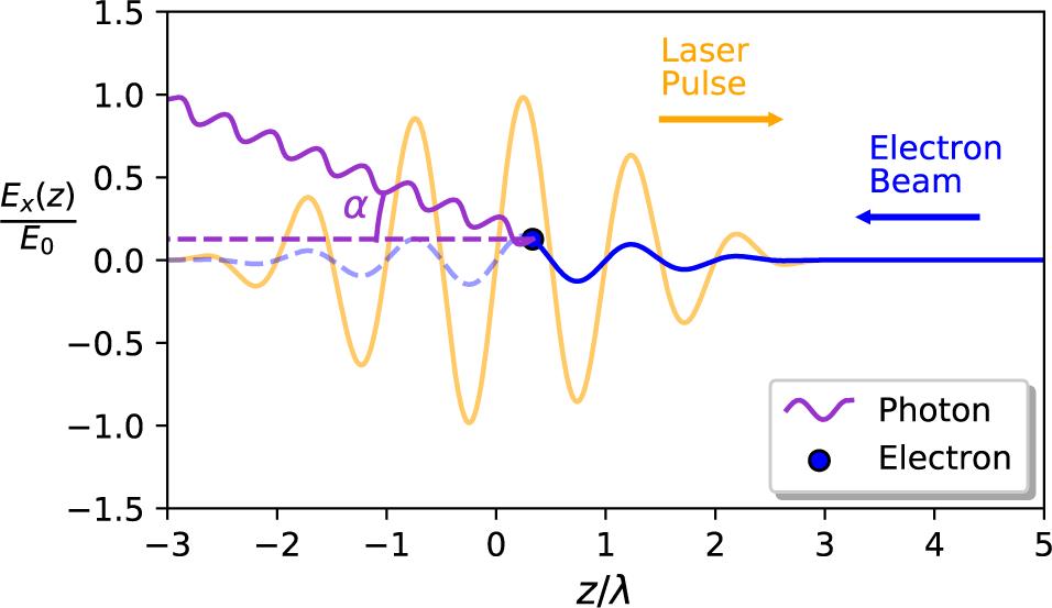
Figure 1.Representation of the numerical implementation of the experiment in which  denotes the peak electric field amplitude (the deviation angle is exaggerated).
It was concluded in Section 2 that the fractional energy distribution
Now, let us try to select a set of moments such that any combination
![]()
Figure 2.Contours of  as a function of
  and
and  where (a) compares
  and
and  and (b) compares
  and
and  .
.
Note that for a larger number of model parameters (representing both theory inquiries and latent parameters of collisions) one would need to inspect the dependency of summary statistics in a multidimensional space, which can be unfeasible. In this case one might need physics insights to make an educated strategy to disentangle specific types of degeneracy. In the considered case we can interpret the identified choice through the following logic. The value of
Let us now continue the analysis for the chosen summary statistics. We make the following choice of priors over
During sampling, the following distance is calculated to discriminate between observations:
In Figure 3 we present the result of sampling the posterior based on the described ABC routine after processing
![]()
Figure 3.The approximate posterior after processing  observations in line with Algorithm 3, where in the bottom panel the dashed line demarcates the sample mean. All distributions have
  accepted proposals.
Having discussed the use of ABCs via the selected proof-of-principle case, we can outline further developments that could help to deal with real experiments. The first direction of developments concerns the elaboration of an appropriate model of experiments, which implies a relevant 3D geometry of interaction with an account of unmeasured variations via an extended list of latent parameters, such as all spatio-temporal offsets, as well as parameters quantifying both the electron bunch and the focused laser pulse. The second direction of developments concerns computational methods to deal with the chosen geometry of the experiment, as well as accounting for all physical processes of relevance, such as the generation of electron–positron pairs and the interaction between particles and photons. Efficient use of supercomputer resources can be crucial to compensate for the increase of computational demands in relation to both the complexity of simulations and the necessity to obtain a meaningfully narrow posterior using a large number of collisions. The third direction of developments concerns improvements related to the use of the ABC itself. This may include a better choice of summary statistics, a modification of diagnostics or the experiment layout, as well as reducing the rejection rate by employing machine learning methods for an informed generation of proposals. Finally, the fourth direction of developments concerns the very formulation of theoretical questions, which takes the form of determining models and parameters to be inferred from experiments.
5 Conclusions
We have considered prospects for an experiment capable of inferring a parameter
References
[1] J. M. Cole, K. T. Behm, E. Gerstmayr, T. G. Blackburn, J. C. Wood, C. D. Baird, M. J. Duff, C. Harvey, A. Ilderton, A. S. Joglekar, K. Krushelnick, S. Kuschel, M. Marklund, P. McKenna, C. D. Murphy, K. Poder, C. P. Ridgers, G. M. Samarin, G. Sarri, D. R. Symes, A. G. R. Thomas, J. Warwick, M. Zepf, Z. Najmudin, S. P. D. Mangles. Phys. Rev. X, 8, 011020(2018).
[2] K. Poder, M. Tamburini, G. Sarri, A. Di Piazza, S. Kuschel, C. D. Baird, K. Behm, S. Bohlen, J. M. Cole, D. J. Corvan, M. Duff, E. Gerstmayr, C. H. Keitel, K. Krushelnick, S. P. D. Mangles, P. McKenna, C. D. Murphy, Z. Najmudin, C. P. Ridgers, G. M. Samarin, D. R. Symes, A. G. R. Thomas, J. Warwick, M. Zepf. Phys. Rev. X, 8, 031004(2018).
[3] H. Abramowicz, U. Acosta, M. Altarelli, R. Aßmann, Z. Bai, T. Behnke, Y. Benhammou, T. Blackburn, S. Boogert, O. Borysov, M. Borysova, R. Brinkmann, M. Bruschi, F. Burkart, K. Büßer, N. Cavanagh, O. Davidi, W. Decking, U. Dosselli, N. Elkina, A. Fedotov, M. Firlej, T. Fiutowski, K. Fleck, M. Gostkin, C. Grojean, J. Hallford, H. Harsh, A. Hartin, B. Heinemann, T. Heinzl, L. Helary, M. Hoffmann, S. Huang, X. Huang, M. Idzik, A. Ilderton, R. Jacobs, B. Kämpfer, B. King, H. Lahno, A. Levanon, A. Levy, I. Levy, J. List, W. Lohmann, T. Ma, A. J. Macleod, V. Malka, F. Meloni, A. Mironov, M. Morandin, J. Moron, E. Negodin, G. Perez, I. Pomerantz, R. Pöschl, R. Prasad, F. Quéré, A. Ringwald, C. Rödel, S. Rykovanov, F. Salgado, A. Santra, G. Sarri, A. Sävert, A. Sbrizzi, S. Schmitt, U. Schramm, S. Schuwalow, D. Seipt, L. Shaimerdenova, M. Shchedrolosiev, M. Skakunov, Y. Soreq, M. Streeter, K. Swientek, N. T. Hod, S. Tang, T. Teter, D. Thoden, A. I. Titov, O. Tolbanov, G. Torgrimsson, A. Tyazhev, M. Wing, M. Zanetti, A. Zarubin, K. Zeil, M. Zepf, A. Zhemchukov. Eur. Phys. J. Spec. Top., 230, 2445(2021).
[4] V. Yakimenko, L. Alsberg, E. Bong, G. Bouchard, C. Clarke, C. Emma, S. Green, C. Hast, M. J. Hogan, J. Seabury, N. Lipkowitz, B. O’Shea, D. Storey, G. White, G. Yocky. Phys. Rev. Accel. Beams, 22, 101301(2019).
[5] A. Gonoskov, T. Blackburn, M. Marklund, S. Bulanov. Rev. Mod. Phys., 94, 045001(2022).
[6] C. Bula, K. T. McDonald, E. J. Prebys, C. Bamber, S. Boege, T. Kotseroglou, A. C. Melissinos, D. D. Meyerhofer, W. Ragg, D. L. Burke, R. C. Field, G. Horton-Smith, A. C. Odian, J. E. Spencer, D. Walz, S. C. Berridge, W. M. Bugg, K. Shmakov, A. W. Weidemann. Phys. Rev. Lett., 76, 3116(1996).
[7] M. Iinuma, K. Matsukado, I. Endo, M. Hashida, K. Hayashi, A. Kohara, F. Matsumoto, Y. Nakanishi, S. Sakabe, S. Shimizu, T. Tauchi, K. Yamamoto, T. Takahashi. Phys. Lett. A, 346, 255(2005).
[8] T. Kumita, Y. Kamiya, M. Babzien, I. Ben-Zvi, K. Kusche, I. V. Pavlishin, I. V. Pogorelsky, D. P. Siddons, V. Yakimenko, T. Hirose, T. Omori, J. Urakawa, K. Yokoya, D. Cline, F. Zhou. Laser Phys., 16, 267(2006).
[9] T. Englert, E. Rinehart. Phys. Rev. A, 28, 1539(1983).
[11] T. Ritto, S. Beregi, D. Barton. Mech. Syst. Sig. Process., 181, 109485(2022).
[12] M. C. Kennedy, A. O’Hagan, J. Roy. Stat. Soc. Ser. B, 63, 425(2001).
[13] D. N. DeJong, B. F. Ingram, C. H. Whiteman. J. Business Econ. Stat., 14(1996).
[14] J. Brehmer, G. Louppe, J. Pavez, K. Cranmer. Proc. Natl. Acad. Sci. U. S. A., 117, 5242(2020).
[15] J. Akeret, A. Refregier, A. Amara, S. Seehars, C. Hasner. J. Cosmol. Astropart. Phys., 2015, 043(2015).
[16] V. Yakimenko, S. Meuren, F. Del Gaudio, C. Baumann, A. Fedotov, F. Fiuza, T. Grismayer, M. J. Hogan, A. Pukhov, L. O. Silva, G. White. Phys. Rev. Lett., 122, 190404(2019).
[17] V. Ritus. Sov. Phys. JETP, 30, 052805(1970).
[18] S. Meuren, A. Di Piazza. Phys. Rev. Lett., 107, 260401(2011).
[19] N. B. Narozhny. Phys. Rev. D, 21, 1176(1980).
[20] V. B. Berestetskii, E. M. Lifshitz, L. P. Pitaevskii. Quantum Electrodynamics(1982).
[21] V. Baier, V. Katkov. Phys. Lett. A, 25, 492(1967).
[22] C. Olofsson, A. Gonoskov. Phys. Rev. A, 106, 063512(2022).
[23] D. E. Rivas, A. Borot, D. E. Cardenas, G. Marcus, X. Gu, D. Herrmann, J. Xu, J. Tan, D. Kormin, G. Ma, W. Dallari, G. D. Tsakiris, I. B. Földes, S. W. Chou, M. Weidman, B. Bergues, T. Wittmann, H. Schröder, P. Tzallas, D. Charalambidis, O. Razskazovskaya, V. Pervak, F. Krausz, L. Veisz. Sci. Rep., 7, 5224(2017).
[24] L. D. Landau. The Classical Theory of Fields(2013).
[25] S. T. Tokdar, R. E. Kass. Wiley Interdisc. Rev. Comput. Stat., 2, 54(2010).
[26] A. Doucet, N. D. Freitas, N. Gordon. Sequential Monte Carlo Methods in Practice, 3-14(2001).
[27] S. Brooks, A. Gelman, G. Jones, X.-L. Meng. Handbook of Markov Chain Monte Carlo(2011).
[28] S. A. Sisson, Y. Fan, M. Beaumont. Handbook of Approximate Bayesian Computation(2018).
[29] K. Cranmer, J. Brehmer, G. Louppe. Proc. Natl. Acad. Sci. U. S. A., 117, 30055(2020).

Set citation alerts for the article
Please enter your email address
© Copyright 2018-2021 | Chinese Laser Press. All Rights Reserved 沪ICP备15018463号-20