Generation of tail-free short pulses using high-pressure CO2 laser

Yue Lu; Ziren Zhu; Jinzhou Bai; Xinjun Su; Rongqing Tan; Jinghan Ye; Yijun Zheng

doi:10.3788/COL202220.051401

Abstract

The spectral linewidth of a transversely excited pulsed

{CO}_{2}

laser is broadened at high working pressures. This phenomenon causes a decrease in the upper-level lifetime such that the pulse width is significantly compressed. Although the tail part of

{CO}_{2}

laser pulses owns a non-negligible proportion of total energy, it has minor effects during the interaction process between photons and materials due to its low amplitude. Thus, it is of great significance to yield the tail part and generate a narrow pulse in most applications. In this study, a continuously tunable pulsed

{CO}_{2}

laser with a low nitrogen proportion in the mixture is developed to generate tail-free short pulses; a minimum pulse width of 30.60 ns with a maximum pulse energy of 481 mJ is synchronously achieved at a pressure of 7 atm, and the estimated peak power is above 15 MW. A numerical simulation is also conducted for comparison with the experimental results. The contribution of the spectral gain toward the compression of the pulse width is discussed in the last section of this paper.

Keywords

continuous tuning pulse compression short pulse

1. Introduction

The generation of short ${CO}_{2}$ laser pulses is presently a frontier research topic. It has wide applications in domains such as laser manufacturing^[1–3], spectrum detection ( ${CO}_{2}$ LIDAR)^[4–6], medical treatments^[7], and military applications^[8]. Moreover, because of the continuously tunable output spectrum, it can be used in laser-induced nuclear fusion^[9,10] and laser isotope separation^[11,12].

A free-running ${CO}_{2}$ laser typically produces sub-microsecond pulses with a considerable proportion of nitrogen tail, which impedes the interacting efficiency of matter. Therefore, various methods, including mode-locking^[13], $Q$ -switching^[14], and filling with a high-pressure gas mixture, have been developed for generating tail-free short pulses. Among these methods, the high-pressure method is regarded as an ideal combination of lower insertion loss and flexible tuning properties. Currently, the shortest high-pressure ${CO}_{2}$ laser pulse width reported is approximately 60 ns^[15]. In this study, a tail-free short pulse was generated using a continuously tunable high-pressure ${CO}_{2}$ laser. Compared with a pulse width of approximately 100 ns at a pressure of 1 atm (standard atmosphere), the pulse width was compressed to a new mean record of approximately 32 ns at a pressure of 7 atm to achieve a maximum compression ratio of 60%. The contribution of the spectral gain toward the compression of the pulse is discussed separately between frequencies for the first time, to the best of our knowledge.

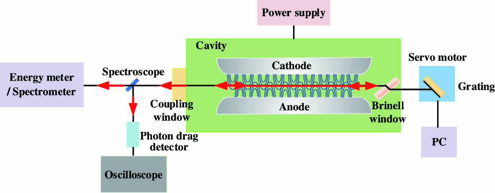
2. Experimental Apparatus

The experimental devices used in this study are illustrated in Fig. 1. The ${CO}_{2}$ laser comprised a sealed chamber and a resonant cavity. The pre-ionization structures and main discharge electrodes were present inside the chamber. Pre-ionization structures are point discharging spark arrays laid along two sides of the discharging area. A pair of Chang profile electrodes was used to obtain a uniform discharge. The cavity length and gain length were 1.2 and 0.6 m, respectively. The gain volume was $10 mm \times 10 mm \times 600 mm$ . The contents of the filled gas mixture had a proportion of ${CO}_{2} : N_{2} : He = 2 : 1 : 16$ . The resonant cavity was a plane-concave cavity profile containing an output coupling window (with a reflectivity $R = 60 %$ ) and a grating (with a grating constant $d = 1 / 150 mm$ ) working at the Littrow angle. The ${CO}_{2}$ laser was pumped using a high-voltage ( $\geq 60 kV$ ) pulsed power source (with an energy capacitor of 7.67 nF) and worked at a repetition rate of 1 Hz. The grating was driven by a servo motor controlled by a personal computer (PC), thus realizing a tunable output.

Sign up for Chinese Optics Letters TOC. Get the latest issue of Chinese Optics Letters delivered right to you！Sign up now

Figure 1.Schematic of the experimental device.

A generated pulse was split using a spectroscope ( $reflectance / transmittance = 1 / 4$ ) such that the pulse energy and pulse width could be collected by an energy meter and photon drag detector simultaneously. When the working angle of the grating was changed, the energy meter could be temporarily replaced by a spectrometer to confirm the output wavelength. In this study, the mentioned pulse energy refers to the numerically converted original value based on the splitting ratio.

3. Theoretical Model

3.1. Six-temperature model

The theoretical models describing the ${CO}_{2}$ molecular dynamic process include the four-temperature model^[16], five-temperature model^[17], and widely adopted six-temperature model (6-T model)^[18]. In contrast to the former models, the contribution of the ${CO}_{2}$ molecular process in achieving level relaxation is included in the 6-T model, and the rotational-level structure of ${CO}_{2}$ molecules is sufficiently considered. Overall, the level structure of the gas mixture is reasonably simplified in this model, considering the effects of long-term operating factors, such as temperature fluctuation and gas decomposition, on the output characteristics as well. The 6-T model reflects the effects of factors such as pre-ionization, discharge cavity size, reflectance of the coupling window, and gas component, which are closely related to the output characteristics.

According to the 6-T model, the magnitudes of energy density in the ${CO}_{2}$ molecular symmetric mode, bending mode, anti-symmetry mode, $N_{2}$ molecular vibration mode, ${CO}_{2}$ molecular vibration mode, and energy during interaction of the ambient mixture are represented as $E_{1}, E_{2}, E_{3}, E_{4}, E_{5}$ , and $E$ , respectively, as illustrated in Fig. 2. Integrating the equations over a period of microseconds, the dynamic progress of the pulsed ${CO}_{2}$ laser can be simulated.

The laser light intensity consists of three parts: the contribution of stimulated radiation, the contribution of spontaneous radiation, and the attenuation caused by loss. $E_{1}$ , $E_{2}$ , $E_{3}$ , $E_{4}$ , and $E_{5}$ represent the energy density of the symmetric stretch mode (the lower level of 10P and 10R), bending mode (the lower level of 9P and 9R), asymmetric stretch mode (the upper level), the first excited state level of $N_{2}$ (close resonance), and the energy level of $CO$ . $X_{1}$ , $X_{2}$ , $X_{3}$ , $X_{4}$ , and $X_{5}$ represent the discharge-pumped effective electron excitation rate. $τ_{α, β}$ ( $α, β = 0$ , 1, 2, 3, 4, or 5) means time constants of relaxation between different energy levels. $ν_{i}$ ( $i = 0$ , 1, 2, 3, 4, or 5) means different frequency components. $N_{{CO}_{2}}$ is defined as the density of ${CO}_{2}$ . $F$ is the fill factor, equal to the ratio of gain length to cavity length.

The detailed rate equations describing energy relaxation between different levels can refer to the works by former researchers^[18–21].

The output power can be expressed as $P_{i} = - \frac{π}{8} D_{M}^{2} F \ln (R T_{r}) \frac{1 - R - K_{M}}{1 - R T_{r}} h c ν_{i} Q_{i} .$ (1)

$D_{M}$ , $R$ , $K_{M}$ , $T_{r}$ , and $Q_{i}$ represent minimum clear aperture, reflectance of coupling window, total diffraction loss, transmittance of resonant cavity, and photon density of single frequency $ν_{i}$ , respectively.

3.2. Theoretical simulation

Because it is difficult to achieve analytical solutions of rate equations, the fourth-order Runge–Kutta algorithm was adopted to calculate the numerical values balancing the accuracy and efficiency. The specific algorithm appropriate for pulsed ${CO}_{2}$ lasers was referred from a previous work^[19].

The simulated weighted forms are presented as follows: $E_{i {n q}}$ , $K_{E_{i {n q}_1}}$ , $K_{E_{i {n q}_2}}$ , $K_{E_{i {n q}_3}}$ , and $K_{E_{i {n q}_4}}$ represent the weighted sum and fitted slopes, and $q$ represents the time unit (calculated unit time length): $E_{i {n q}} = E_{i {(n - 1) q}} + \frac{q}{6} (K_{E_{i {n q}_1}} + 2 K_{E_{i {n q}_2}} + 2 K_{E_{i {n q}_3}} + K_{E_{i {n q}_4}}),$ (2) $K_{E_{i {n q}_1}} = \frac{d E_{i}}{d t} [t = (n - 1) q],$ (3) $K_{E_{i {n q}_2}} = \frac{d E_{i}}{d t} [t = (n - 1) q + \frac{q}{2} K_{E_{i {n q}_1}}],$ (4) $K_{E_{i {n q}_3}} = \frac{d E_{i}}{d t} [t = (n - 1) q + \frac{q}{2} K_{E_{i {n q}_2}}],$ (5) $K_{E_{i {n q}_4}} = \frac{d E_{i}}{d t} [t = (n - 1) q + q K_{E_{i {n q}_3}}] .$ (6)

The main parameters (the gas pressure was considered as a variable) used in the program include: (a)gas mixture: ${CO}_{2} : N_{2} : He = 2 : 1 : 16$ ,(b)reflectance of the coupling window, $R = 60 %$ ,(c)effective aperture of 12 mm,(d)gain length/cavity length of 0.6 m/1.2 m.

4. Statistics and Discussion

Pulse width is closely related to factors such as total injection, pre-ionization intensity, gas pressure, and mixture proportion. Limited experimental conditions can be adopted for achieving a uniform glowing discharge in a large area at high atmospheric pressure. Thus, suitable mixture proportions and discharge parameters were determined through a series of statistical filtrations. In this work, the mixture proportion was ${CO}_{2} : N_{2} : He = 2 : 1 : 16$ , total discharge capacitance (containing pre-ionization discharge capacitance) was 7.67 nF, and discharge voltage varied with the gas pressure setting as follows: 57, 60, 63, and 66 kV at 4, 5, 6, and 7 atm, respectively. Only gas pressure was considered for the pulse width, and the distribution characteristics between the lines in the total output frequency spectrum are discussed.

4.1. Waveform

Figures 3 and 4 depict the experimental and theoretical pulse forms, respectively, of 10P(20) at different pressures. In the vertical axis, the amplitude cell spacing is set as 20 mV in Fig. 3(a), 50 mV in Figs. 3(b) and 3(c), and 100 mV in Fig. 3(d). In the horizontal axis, the time cell spacing is set as 100 ns. Clearly, there was a significant increase in peak power with an increase in pressure and a reduction in pulse width. According to the formula $P τ = C$ ^[19], the pressure is inversely proportional to the upper-level lifetime, and the experimental pulse width decreases at a higher pressure.

Figure 2.Six-temperature model CO₂-N₂-CO gas pump energy-level diagram.

Figure 3.Experimental pulse forms and amplitudes at different pressures: (a) 4 atm, 130 mV, (b) 5 atm, 280 mV, (c) 6 atm, 370 mV, and (d) 7 atm, 550 mV.

Figure 4.Simulated pulse forms at different pressures.

The theoretical results reflect the same tendency and predict an increase in pulse energy (see Table 1).

Gas pressure (atm)	Pulse width (ns)	Energy (mJ)
4	48.8	196.2
5	39.2	272.7
6	36.7	403.4
7	30.4	493.7

Table 1. Pulse Widths and Corresponding Energy Values at Different Gas Pressures

View all Tables

A comparison of the pulse compression effects at different pressures is plotted in Fig. 4. The experimental compression ratio at 4 atm was 56% of that at 7 atm, whereas the theoretical ratio was 55%.

The experimental pulse forms exhibited a tail-free shape unlike the theoretical forms, which probably causes a difference in the calculated pulse width. It should be noted that an empirical equation representing the density of pumping electrons was adopted in the 6-T model^[19]: $N_{e} (t) = N_{0} \exp (- \frac{t}{t_{A}}) [1 - \exp (- \frac{t}{t_{B}})] .$ (7)

$t_{A}$ and $t_{B}$ are optimized to make a similar simulation according to the realistic discharging waveform. Some details like inflection points hardly match the experimental data, which may cause the discrepancy in symmetry. Therefore, there may be a tiny tail in the simulation form, and the main body of such a pulse is narrower.

Experimental values of pulse width are related to many factors. Three main factors are mentioned below. Firstly, this uncertainty is owing to the electrical desynchrony of the discharging process controlled by high-voltage capacitors and switches. On the other hand, density of electrons has unavoidable fluctuations in the discharging process due to the stochastic plasma diffusion. Thirdly, theoretical models considered an ideal system without thermal deposition, while it commonly exists in real discharging cavities. These factors closely affect the rising and falling edges in the laser gain curve so that the pulse widths do have different values (see Fig. 5).

Figure 5.Theoretical and experimental pulse widths at different pressures [10P(20)].

The differences of the pulse shapes and widths between simulated and experimental ones may be a limitation of the current 6-T model.

4.2. Pulse width and pulse energy

As shown in Fig. 6, the pulse width varied with the frequencies of different output bands. This is essentially affected by the stimulated emission cross section of the upper and lower levels. The oscillating frequencies in the central portion exhibited a higher gain than those at the two ends of the same band. The threshold conditions for laser output are highly available at these preponderant frequencies and also at the abrupt rising edge of the pulse form and higher pulse energy. Consequently, the distributions of the pulse width and energy over the entire spectrum presented opposite-shaped graphs resembling a regular “V” and an inverted “V,” respectively.

Figure 6.Normalized pulse width and energy versus wavelength (7 atm).

4.3. Pulse width at different pressures

Figure 7 depicts the pulse width distributions for different output bands at various mixture pressures. With an increase in pressure, four statistical observations were made. (a)The entire pulse width decreased in all bands. Considering 10P(20) as an example, the pulse widths varied from 55.9 ns (4 atm) to 35.7 ns (7 atm), owing to the higher pressure and discharge voltage caused by the larger injection and total gain.(b)Similarly, a larger total gain resulted in an increased gain in the marginal frequencies of the current band, and the output frequency spectrum was reasonably extended. For example, in the 9R band, the range of the output wavelength at 4 atm was 9.25–9.31 µm, and it expanded from 9.21 to 9.31 µm at 7 atm.(c)The difference between the frequencies in a single band diminished with the mixture pressure. For 10R(18), maximum difference values of 77.6 and 39.4 ns were obtained at 4 and 7 atm, respectively. Collision broadening mainly leads to the spectral broadening in high-pressure ${CO}_{2}$ lasers, which corresponded to the superior modulation degree of the distribution of energy over the entire output spectrum¹⁹.(d)Different bands exhibited different compression ratios at different pressures. Figure 6 shows that the pulse width of the 10P band exhibited compressions from 90.40 to 59.73 ns at maximum and from 63.11 to 39.39 ns at minimum. Figure 7 also shows that the pulse width of the 9R band exhibited compressions from 76.10 to 52.40 ns at maximum and from 42.20 to 32.13 ns at minimum. The total difference between the bands likely contributed to this phenomenon, similar to the explanation given in (c). When the pressure was lower (4 atm), the output of the marginal frequencies, such as 9P, wandered around the gain switch and exhibited a relatively larger pulse width, while 10P resulted in a considerably higher gain. When the total gain substantially increased with the pressure, the pulse width of the lines of 9P was compressed by a large scale, and the originally preponderant lines of bands such as 10P reached a gain saturation and exhibited a comparatively insignificant change in the pulse width.

Figure 7.Pulse widths of 9R, 9P, 10R, and 10P versus wavelength.

5. Conclusion

In this work, by increasing the working pressure of a ${CO}_{2}$ laser, a continuously tunable output was realized at a pressure of 7 atm. The mixture ratio was ${CO}_{2} : N_{2} : He = 2 : 1 : 16$ , discharge voltage was 66 kV, energy storage capacitance was 7.67 nF, and output coupling window reflectance was $R = 60 %$ . The shortest mean pulse width of 30.60 ns with a peak power $> 15 MW$ and a pulse energy of 481 mJ was achieved at line 9R(20), and a mean pulse width of 35.70 ns with a pulse energy of 391 mJ was achieved at line 10P(20). Compared with the pulsed high-pressure ${CO}_{2}$ laser with a similar injection, the pulse width reached a scale of nearly 50%^[15].

In addition, three types of differences were discussed in the previous section, namely the statistical differences between the experimental and theoretical data, differences between the pulse width and pulse energy distributions, and differences between the pulse widths at different bands and different frequencies. First, it was revealed that the experimental results and theoretical simulations demonstrated corresponding regularity. Second, the distributions of pulse width and pulse energy exhibited opposite graph shapes. Third, the pulse width was compressed, and the differences between bands and frequencies diminished with an increase in the working pressure.

The scope of future work includes conducting more specific theoretical expressions connecting basic parameters with spectral distribution properties of pulse width, and a series of parametric optimizations to be carried out at higher pressures. Results of this paper will make further improvements in aspects such as mode selecting technique in continuously wavelength tunable single longitudinal mode lasers, $Q$ -switching technique on generating ultrashort pulses under picoseconds, quasi-phasing-matching technique in acquiring frequency-doubling laser pulses, and isotopic separation technique by stimulated Raman scattering lasers.

References

[1] D. Holder, A. Leis, M. Buser, R. Weber, T. Graf. High-quality net shape geometries from additively manufactured parts using closed-loop controlled ablation with ultrashort laser pulses. Adv. Opt. Technol., 9, 101(2020).

[2] H. Büttner, K. Michael, J. Gysel, P. Gugger, S. Saurenmann, G. de Bortoli, J. Stirnimann, K. Wegener. Innovative micro-tool manufacturing using ultra-short pulse laser ablation. J. Mater. Process. Technol., 285, 116766(2020).

[3] B. Huis in ’t Veld, L. Overmeyer, M. Schmidt, K. Wegener, A. Malshe, P. Bartolo. Micro additive manufacturing using ultra short laser pulses. CIRP Ann. Manuf. Technol., 64, 701(2015).

[4] P. P. Geiko, A. Tikhomirov. Remote measurement of chemical warfare agents by differential absorption CO2 lidar. Opt. Mem. Neural Netw., 20, 71(2011).

[5] D. C. Dumitras, S. Banita, A. M. Bratu, R. Cernat, D. C. A. Dutu, C. Matei, M. Patachia, M. Petrus, C. Popa. Ultrasensitive CO2 laser photoacoustic system. Infrared Phys. Technol., 53, 308(2010).

[6] P. P. Geiko, A. Tikhomirov. Remote measurement of chemical warfare agents by differential absorption CO2 lidar. Opt. Mem. Neural Netw., 20, 71(2011).

[7] S. Nikiforov, Y. Simanovsky, A. Pento, K. Moshkunov, N. Gorbatova, S. Zolotov, S. Alimpiev. Pulsed transverse discharge CO2 laser for medical applications. International Conference Laser Optics (LO)(2016).

[8] R. H. M. A. Schleijpen, F. J. M. van Putten. Using a CO2 laser for PIR-detector spoofing. Proc. SPIE, 9989, 99890K(2016).

[9] Y. Zhang, H. Wang, L. Liu, Y. Ma, B. Shen, G. Zhang, M. Huang, A. Bonasera, W. Wang, J. Xu, S. Li, G. Fan, X. Cao, Y. Yu, C. Fu, J. He, S. Zhang, X. Hu, X. Li, Z. Hao, J. Wang, H. Xue, H. Fu. Primary yields of protons measured using CR-39 in laser-induced deuteron–deuteron fusion reactions. Nucl. Sci. Tech., 31, 62(2020).

[10] S. S. Perrotta, A. Bonasera. Fusion hindrance effects in laser-induced non-neutral plasmas. Nucl. Phys. A, 989, 168(2019).

[11] R. Snyder. A proliferation assessment of third generation laser uranium enrichment technology. Sci. Glob. Sec., 24, 68(2016).

[12] V. K. Saini, S. Talwar, V. V. V. Subrahmanyam, S. K. Dixit. Laser assisted isotope separation of lithium by two-step photoionization using time of flight mass-spectrometer. Opt. Laser Technol., 111, 754(2019).

[13] J. C. Balzer, T. Schlauch, A. Klehr, G. Erbert. High peak power pulses from dispersion optimized mode-locked semiconductor laser. Electron. Lett., 49, 838(2013).

[14] Y. R. Yuzaile, N. A. Awang, N. U. H. H. Zalkepali, Z. Zakaria, A. A. Latif, A. N. Azmi, F. S. Abdul Hadi. Pulse compression in Q-switched fiber laser by using platinum as saturable absorber. Optik, 179, 977(2019).

[15] H. V. Bergmann, F. Morkel. Continuously wavelength tunable high pressure CO2 lasers. Proc. SPIE, 9255, 92551Y(2015).

[16] J. Gilbert, J. L. Lachambre, F. Rheault, R. Fortin. Dynamics of the CO2 atmospheric pressure laser with transverse pulse excitation. Can. J. Phys., 50, 2523(1972).

[17] K. J. Andrews, P. E. Dyer, D. J. James. A rate equation model for the design of TEA CO2 oscillators. J. Phys. E, 8, 493(1975).

[18] O. Richter, R. Seppelt, D. Sndgerath. Computer Modeling(2006).

[19] J. N. Elgin. Computer modeling of gas lasers. Electron. Power UK, 25, 441(1979).

[20] M. Kimmit. Book Review: The CO2 laser. By W. J. Witteman. Springer Series in Optical Sciences, Vol. 53. Springer-Verlag, 1987. 309 pp. Price: DM 98 (hard cover). Opt. Lasers Eng., 11, 66(1989).

[21] A. R. Davies, K. Smith, R. M. Thomson. TLASER—a CO2 laser kinetics code. Comput. Phys. Commun., 10, 117(1975).