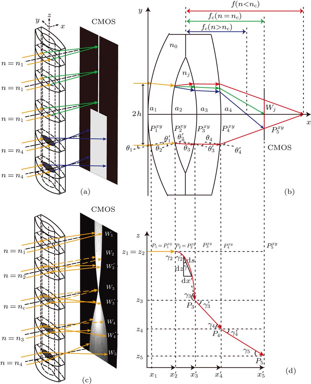
Fig. 1. (a) Three-dimensional (3D) imaging diagram of ray in homogeneous media, (b) 3D imaging diagram of ray in inhomogeneous media, (c) two-dimensional (2D) imaging diagram of ray in homogeneous media (xy plane), and (d) 2D imaging diagram of ray in inhomogeneous media (x’z plane).

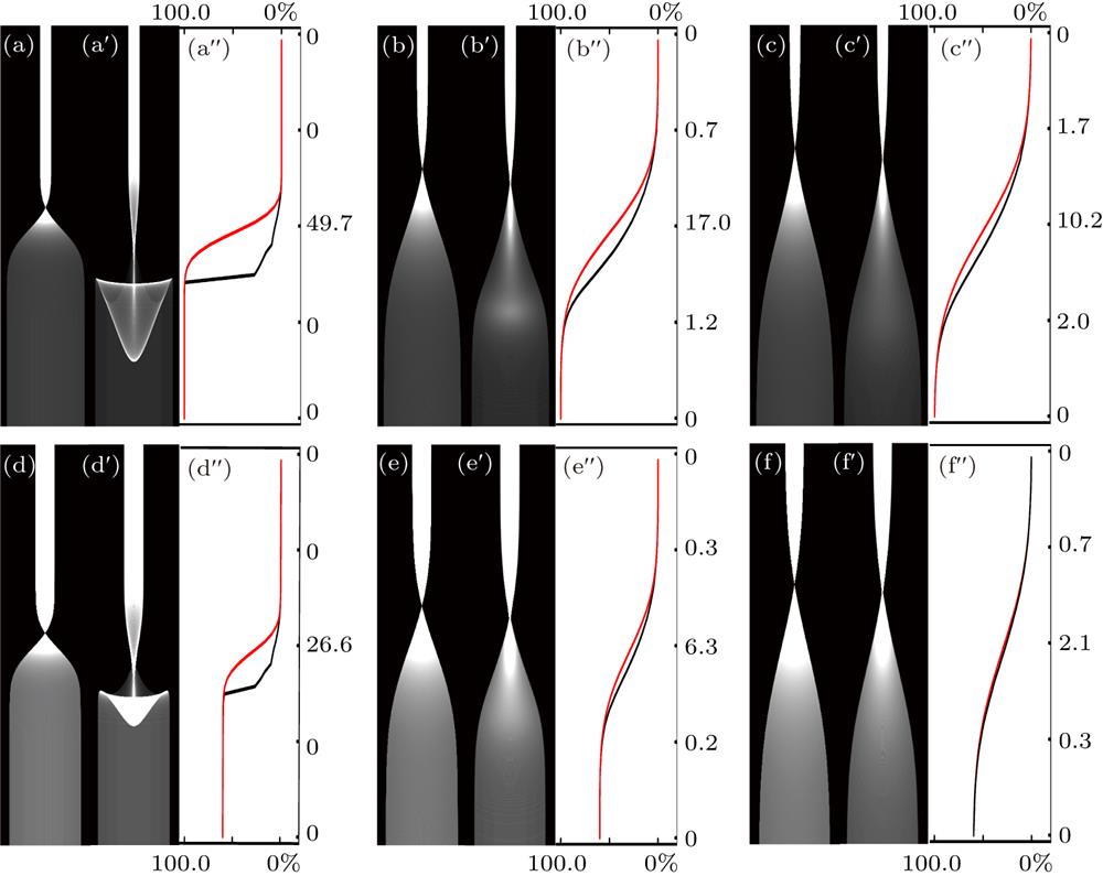
Fig. 2. Comparison between two simulated results. (a)–(f): Simulated diffusion images in “homogeneous media”, where (a), (b), (c): C₂ – C₁ = 1.0, t = 20, 150, 270 min; (d), (e), (f): C₂ – C₁ = 0.6, t = 20, 150, 270 min; (a′)–(f′): simulated diffusion images in inhomogeneous media; (a″)–(f″) the concentration relative deviations of two kinds of simulations.

Fig. 3. Typical experimental diffusion images for [(a) and (b)] 0%–60% diffusion group at t = 320 min (a) and 380 min (b), and [(c) and (d)] 40%–10% diffusion group at t = 450 min (c) and 540 min (d).

Fig. 4. Spatial and temporal concentration profiles C^e(z_j, t)s corresponding to Fig. 3, at t = 320 min (a), 380 min (b), 450 min (c), and 540 min (d), with rectangular points representing experimental values, and solid red lines denoting calculated values.

Fig. 5. Comparison of D(C) between measured values and literature values. Red empty circle represents measured value of D₁(C) in concentration range of 0%–60%. Solid red circle denotes measured value of D₂(C) in concentration range of 40%–100%. Solid line refers to fitting curve D(C) in concentration range of 0%–100%. Upper triangle represents measured values of literature 1. Lower triangles are for measured values of literature 2. Error bars, which are magnified 5 times for the sake of clarity, are determined by ten-time independent measurements.

Fig. 6. Comparison between experimental diffusion images and simulated images at RI = n_c = 1.3482 for the first diffusion group (0%–60%): [(a′), (b′), (c′)] experimental diffusion images at t = 25, 210, and 380 min; [(a), (b), (c)] simulated images in “homogeneous solution”; [(a″, b″, c″)]: simulated images in inhomogeneous solution. Longitudinal scales represent solution concentrations.

Fig. 7. Comparison between experimental diffusion images and simulated images at RI = n_c = 1.3994 for the second diffusion group (40%–100%): [(a′), (b′), (c′)] experimental diffusion images at t = 40, 360, and 540 min; [(a), (b), (c)] simulated images in “homogeneous solution”; [(a″), (b″), (c″)] simulated images in inhomogeneous solution. Longitudinal scales represent solution concentrations.

Table 1. Measurement and calculation results of D(C) in a range of 0%–60% concentration.

Table 2. Measurement and calculation results of D(C) in a range of 40%–100% concentration.