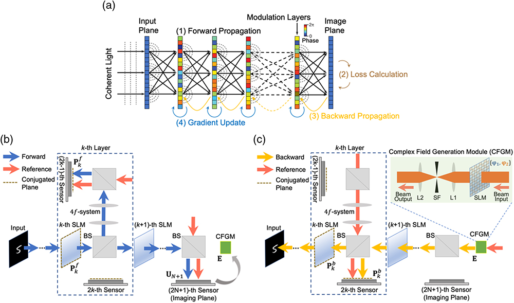
Fig. 1. Optical training of diffractive ONN. (a) The diffractive ONN architecture is physically implemented by cascading spatial light modulators (SLMs), which can be programmed for tuning diffractive coefficients of the network towards a specific task. The programmable capability makes it possible for in situ optical training of diffractive ONNs with error backpropagation algorithms. Each iteration of the training for updating the phase modulation coefficients of diffractive layers includes four steps: forward propagation, error calculation, backward propagation, and gradient update. (b) The forward propagated optical field is modulated by the phase coefficients of multilayer SLMs and measured by the image sensors with phase-shifted reference beams at the output image plane as well as at the individual layers. The image sensor is set to be conjugated to the diffractive layer relayed by a 1:1 beam splitter (BS) and a 4f system. (c) The backward propagated optical field is formed by propagating the error optical field from the output image plane back to the input plane with the modulation of multilayer SLMs. The error optical field is generated from the complex field generation module (CFGM) by calculating the residual errors between the network output optical field and the ground truth label. With the measured forward and backward propagated optical fields, the gradients of the diffractive layers are calculated, and the modulation coefficients of SLMs are successively updated from the last to first layer.

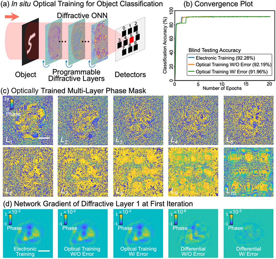
Fig. 2. In situ optical training of the diffractive ONN for object classification on the MNIST dataset. (a) By in situ dynamically adjusting the network coefficients with programmable diffractive layers, the diffractive ONN is optically trained with the MNIST dataset to perform object classification of the handwritten digits. (b) The numerical simulations on 10-layer diffractive ONN show the blind testing classification accuracy of 92.19% and 91.96% for the proposed in situ optical training approach without and with the CFGM error, respectively, which achieves a performance comparable to the electronic training approach (classification accuracy of 92.28%). (c) After the optical training (with CFGM error), phase modulation patterns on 10 different diffractive layers (L1,L2,…,L10) are shown, which are fixed during the inference for performing the classification at the speed of light. (d) The visualization of the network gradient reveals that the proposed optical error backpropagation accurately obtains the network gradient with accuracy comparable to the electronic training by calculating the differential between the electronic and optical gradients of the diffractive layer one at first iteration. Scale bar: 1 mm.

Fig. 3. In situ optical training of the diffractive ONN as an optical matrix-vector multiplier. (a) By encoding the input and output vectors to the input and output planes of the network, respectively, the diffractive ONN can be optically trained as a matrix-vector multiplier to perform an arbitrary matrix operation. (b) A four-layer diffractive ONN is trained as a 16×16 matrix operator [shown in the last column of (c)], the phase modulation patterns (L1,L2,L3,L4) of which are shown and can be reconfigured to achieve different matrices by programming the SLM modulations. (c) With an exemplar input vector on the input plane of the trained network (first column), the network outputs the matrix-vector multiplication result (second column), which achieves comparable results with respect to the ground truth (third column). (d) The relative error between the network output vector and ground truth vector is 1.15%, showing the high accuracy of our optical matrix-vector architecture. (e) By increasing the number of modulation layers, the relative error is decreased, and matrix multiplier accuracy can be further improved. Scale bar: 1 mm.

Fig. 4. Instantaneous imaging through scattering media with in situ optical training of the diffractive ONN. (a) The wavefront of the object is distorted by the scattering media and generates the speckle pattern on the detector under freespace propagation (top row). The diffractive ONN is in situ optically trained to take the distorted optical field as an input and perform the instantaneous de-scattering for object reconstruction (bottom row). (b) The MNIST dataset is used to train a two-layer diffractive ONN. The performance of the trained model is evaluated by calculating the peak signal-to-noise ratio (PSNR) of the de-scattering results on the testing dataset, which increases with the reasonably increasing layer distance. (c) The network de-scattering result on the handwritten digit “9” from the MNIST testing dataset shows PNSRs of 16.9 dB and 30.3 dB at layer distances of 10 cm and 90 cm, respectively. (d) An eight-layer diffractive ONN trained with the Fashion-MNIST dataset successfully reconstructs the objects of “Trouser” and “Coat” (images of the testing dataset) from their distorted optical wavefront. (e) Convergence plots of the two-, four-, and eight-layer diffractive ONN trained with the Fashion-MNIST dataset, which achieves PSNRs of 18.3 dB, 19.3 dB, and 21.2 dB on the testing dataset, respectively. Scale bar: 1 mm.

Fig. 5. Performance of the in situ optically trained MNIST classifier with respect to the number of diffractive layers. The classification accuracy increases with the increase in number of layers. For demonstration and comparison, the layer number of the classification network is set to 10, as shown in Fig. 2 of the main text.

Fig. 6. Performance of the trained optical matrix-vector multiplier with respect to the size of the training set. The training, testing, and validation datasets are generated in an electronic computer by using the target matrix operator as shown in the last column of Fig. 3(c) of the main text, which is used for in situ optical training of the diffractive optical neural network (ONN) to perform the optical matrix-vector multiplier. The dataset’s input vectors are randomly sampled with a uniform distribution between zero and one. With the network settings detailed in Section 4.C of the main text, the convergence plots of the training with different training set sizes are shown in (a), where the relative errors are evaluated over the validation dataset. The performance of the optically trained diffractive ONN with respect to the training set size evaluated on the testing dataset is shown in (b). Although increasing the size of the training set reduces the relative error and improves network performance, it requires more computational resources in an electronic computer. The numerical experimental results show the comparable model accuracy and convergence speed when the training set size is larger than 500, which is therefore adopted for this application. To sufficiently evaluate the generalization of the network, both the validation and testing datasets are set to have a size of 1000.

Fig. 7. Gradient calculation for system calibration under misalignment error. The proposed in situ optical training avoids the accumulation of misalignment error from layer to layer, and the alignment complexity is independent of the network layer number. The misalignment of our in situ optical training is evaluated by including different amounts of misalignment between the measurements of the forward and backward optical fields at each layer. To calibrate the system at each layer, the symmetrical Gaussian phase profile (a) is used as the calibration pattern on the spatial light modulator. The calibration process is to optically calculate the gradient of the diffractive layer given the uniform input pattern as well as the uniform ground truth measurement for determining the amount of misalignment. Due to the use of symmetrical Gaussian phase modulation, the calculated gradient should also be symmetrical if there is no misalignment error, as shown in the first columns of (d)–(f). The misalignment on the x axis and y axis, e.g., 8 μm, 16 μm, and 32 μm, will cause the corresponding asymmetry of the gradient patterns on the x axis and y axis, as shown in the second, third, and fourth columns of (d)–f), respectively, with the cross-section profiles shown in (b) and (c), where the amount of asymmetry can be used for estimating the amount of misalignment error. The in situ optical training system can be calibrated by minimizing the asymmetry of the gradient pattern at each layer. Scale bar: 200 μm.

Fig. 8. In situ optical training of nonlinear diffractive ONN. (a) The optical nonlinearity layer is incorporated into the proposed architecture by using the ferroelectric thin film [23] to perform the activation function for individual layers. (b) To calculate the optical gradient for the nonlinear diffractive ONN, the optical fields are measured for both diffractive and nonlinear layers during forward propagation. (c), (d) Backward propagation is divided into two steps, i.e., backward propagating the error optical field and modulation field separately.

Fig. 9. Convergence plot of the nonlinear diffractive ONN for object classification on the MNIST dataset in comparison with the linear diffractive ONN in Section 4.A of the main text.

Table 1. Computational Performance of the Proposed Optical Training Architecture^a