Generally, defocused images need to be avoided, especially for particle measurements using traditional imaging methods, such as optical microscopy^[1], particle image velocimetry^[2], and particle tracking velocimetry^[3]. To achieve this, the measuring volume is usually limited to the depth of field (DOF) of the imaging system by using light-sheet illumination^[4]. But, defocusing phenomena are unavoidable in in-line measurements^[5], and the DOF is very limited for systems with higher resolutions or magnifications, such as optical microscopy imaging, since DOF is inversely proportional to the magnification of a lens. The usual methods of getting the three-dimensional (3D) positions of an object include holography^[6] and binocular vision^[7]. The former one is a promising method yet still in development. For the latter method, a population of particles is randomly distributed in the measuring volume, and the most important and difficult problem is the matching algorithm in image processing.

Positions in a two-dimensional (2D) frame can be easily extracted from one 2D image. And the level of defocused blurring of the images indicates the depth information of the objects in the third dimension, but there is a problem of position ambiguity. That is to say, a certain level of defocused blur has two corresponding possible object locations. One is in front of the focused object plane and the other is on the opposite side of it. The unique position is generally obtained using two images captured with different camera parameter settings^[8], but that cannot be used with moving objects. Some researchers also found a way by using one image, such as Yoon and Kim^[9], who used a creative three-pinhole aperture to detect the 3D positions. Depth from defocus (DFD) is still one of the most interesting 3D recovery methods in imaging techniques.

In this Letter, two images with different degrees of defocus were captured at the same time to determine the unique position of the moving particles. In order to get these two images, a special measuring system was proposed and established in our studies. Unlike the method of binocular vision, the moving particles in this new method were measured from the same direction, avoiding complex point spatial matching. The problem of position ambiguity for moving particles can be solved without references by using this method.

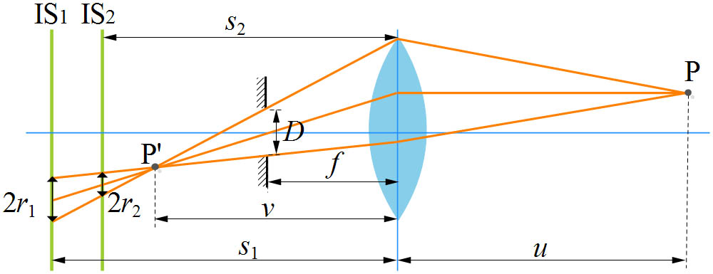
The object-space telecentric lens^[10] is usually used in particle measurements, since the image magnification is independent of the object’s distances or positions. It was adopted here for our theoretical analysis of the DFD principle, which is also suitable for other lenses. Figure 1 shows the schematic drawing of the imaging light path using an object-space telecentric lens with focal length f and aperture size D. A point P at the object distance u has an in-focus image P′ at the image distance v. If two image sensors IS1 and IS2 were located at different image distances s1 and s2, respectively, two circles of confusion with different radii r1 and r2 will be captured.

According to the geometric similarity, the relationship between r1 and r2 can be expressed as Eq. (1), where α is defined as the ratio of blur radius r1 to r2: α≡r1r2=s1−v±s2∓v.(1)

By combining this equation with Gaussian formula 1u+1v=1f, u can be determined by u=f(s1−αs2)s1−f−α(s2−f),(α>1,v<s2<s1α<1,s2<s1<v),(2)u=f(s1+αs2)s1−f+α(s2−f),(s2<v<s1).(3)Equation (2) refers to the condition that the focused image is located at the same side of the two image sensors IS1 and IS2, and Eq. (3) refers to the condition that the focused image is located between these two image sensors. So the first problem is how to distinguish these two conditions and how to determine which equation should be used during the measurement. Secondly, in order to obtain the unique object distance u, the value α should be determined by comparing these two images.

Figure 2 shows five probable locations of the virtual focused image plane with respect to the two real imaging planes. Two conditions, Figs. 2(a) and 2(b), required the focused image plane to be located at the same side of the two image sensors, corresponding to Eq. (2). The condition (Fig. 2(d)) was that the focused images plane was located between the two image sensors, corresponding to Eq. (3). Figures 2(c) and 2(e) show the two critical circumstances in which the focused image plane is located on just one of the image sensors.

When the focused image is located in the image sensor IS2, the radius of dispersion circle r2 is marked as δ1. And when the focused image is located in the image sensor IS1, the radius of dispersion circle r1 is marked as δ2.

According to the geometrical similarity of the imaging system, the radii in the two critical conditions were δ1=D(s1−s2)s2−f,(4)δ2=D(s1−s2)s1−f,(5)both of which were constant for a certain system. During image processing, if the two radii r1 and r2 were, respectively, less than δ1 and δ2, then Eq. (3) will be used; otherwise, Eq. (2) should be used.

Then, the remaining problem is the determination of the blur radius ratio α from these two defocused images. It can be noted that the radius of the dispersion circles or the width of the image edge increases as the level of defocus increases. Substantially, the edges indicated the regions containing a high gradient of gray-level images, or the transition region. For example, M1 and M2 were two images of the same particle with different levels of defocus. The image gradients can be estimated using gradient operators, such as the Sobel operator^[11]. Then, thresholding was performed on the gradient images to get the binary images N1 and N2. In this work, one of the most common algorithms, Otsu’s method^[12], was adopted in the thresholding process. Since the particle images were separated at first and the background gray level was kept constant, this method leads to a constant threshold value. Figure 3 shows the original images and the corresponding binary results of the gradient images.

The white parts in N1 and N2 indicate the transition regions. Let W and C be the area and circumference of the transition regions, respectively. Then, α=r1r2=W1/C1W2/C2.(6)By substituting Eq. (6) into Eq. (2) or (3), the unique object distance u was obtained and the particles would be positioned.

Based on the imaging principle shown in Fig. 1, an imaging system was developed to validate this method. It consisted of one lens (magnification 1×, working distance 65 mm) and two cameras (resolution 1280×1024, pixel size 3.75 μm), as illustrated in Fig. 4. A beam splitter was used to connect the lens and two cameras, and the difference of distances between the two image sensors and the lens (s1 to s2) was 9.1 mm. The distance has an important relationship with the DOF of the lens, and it influences the depth range of the measurement and the corresponding measuring accuracy. A larger difference causes a larger depth range and smaller accuracy. Here, different distances are not discussed, but the measuring principle and method are focused. The synchronous exposure of these two cameras was realized with a signal generator. Two images with different degrees of defocus can be captured for the same moving particles simultaneously. The depth information can then be extracted from these two images using Eq. (2) or (3). However, there were three systematic parameters in these two formulas, f, s1, and s2, which should be determined or calibrated before measurement. On the other hand, the values of parameters δ1 and δ2 were unknown parameters for the equation selection.

The light path in Fig. 1 was applicable to both the thin lens and lens groups, but for the latter one, the object and the image principal planes were not at the same location. Although these parameters are kept confidential by the manufacturers, some of the parameters may be changed for the lens with the beam splitter. (The term “lens-prism group” will be used in the following text to indicate the lens with the beam splitter). Therefore, a calibration method was developed to find the respective parameters, including the focal length f, the location of object’s principal plane, and the location of the image’s principal plane, as shown in Fig. 5. Adapter rings with different thicknesses were used to adjust the distances between the cameras and the lens or lens-prism group from 0 to about 120 mm. For different image distances, the object distance was determined by finding the clearest images as the object moved along the optical axis in intervals of 0.1 mm. An image-processing algorithm that adopted the Sobel operator was developed to quantitatively estimate the degree of defocus. Then, a series of working distances w as image offset distances y can be obtained and used for the estimation of the systematic parameters.

Using the above-mentioned data, the curve fitting was carried out using the Gaussian equation, as shown in Fig. 6. Because it combined a beam splitter, the maximum working distance of the lens-prism group was reduced from 65 to about 43 mm. When the working distance was reduced to lower than 30 mm, it was difficult to find a clear image, so 30 mm was set as the lowest limit. The calibrated parameters of the preliminary lens and the lens-prism group are listed in Table 1, and the results showed that the parameters changed a bit with the beam splitter. L3 largely increased because of the added beam splitter.

Knowing the focal length f and object distances u1 and u2, the distances from the image’s principal plane to the image planes s1 and s2 can be determined with the Gaussian formula. The results showed that s1 was 130.14 mm and s2 was 122.40 mm.

The last problem was the determination of δ1 and δ2. According to Eqs. (4) and (5), D was an unknown parameter, but it was also one of the confidential parameters of the manufacturer. Here, the critical radii were obtained by experiments using the single-lens dual-camera system with certain s1 and s2. A group of images of standard dots along the axis were taken, and the width of transition regions on sensor IS1 or IS2 were detected while the image was focused on the other sensor. Figure 7 shows the respective images of IS1 and IS2 in the two critical circumstances. The values of δ1 and δ2 are 67.0 and 70.1 μm, respectively.

Simulations were performed first to verify the measurement principles and methods of the single-lens dual-camera system. The parameters for simulation were set the same as those in experiments. Figure 8 shows five representative groups of images with different degrees of defocus, indicating different object locations. The disc blur model was used in the simulations. Then, the processing program mentioned above was used to deal with these images, and the result is shown in Table 2.

It is noted from the Table 2 that the calculated results are in good agreement with the real object distances. The results prove that the principle and method are theoretically correct and feasible.

Experimental validations were also performed with the above-mentioned single-lens dual-camera system using a standard dot 2 mm in size. Fifty groups of images were captured when the plate moved along the optical axis in the object distance from 31.5 to 55.5 mm. Four representative groups of images are shown in Fig. 9, and the measurement errors from 50 groups of images were within 4% in the range of 20 times DOF length of the lens, as shown in Fig. 10. The errors increased when the object was far away from the DOF range of the imaging system.

Here, moving bubbles were continuously produced by the electrolysis of salt water in a small, rectangular vessel, as shown in Fig. 11. Bubbles formed on the electrode pole, which was about 30–50 mm away from the lens. A couple of captured images and the corresponding processed results are shown in Fig. 12.

Those two images were taken simultaneously by the two cameras. Three different kinds of particle locations can be detected in the pictures by comparing the degrees of defocus. The red and blue boxes indicate particles where the focused imaging plane was on the same side of IS1 and IS2 and Eq. (2) was used. The particles in the red one were with the focused imaging plane near IS2 (s1>s2>v), and those in the blue one are near IS2 (v>s1>s2). This indicates that the particles in the red box were further from the lens, which is consistent with the processed results. The yellow box indicated particles where the focused imaging plane was located between IS1 and IS2 and the particle positions were also between the above circumstances. The results from the different defocusing conditions indicate the feasibility of this method.

A method for 3D positioning moving particles is proposed by imaging with different imaging distances. To solve the problems caused by particle movement, a single-lens dual-camera system is designed and the calibration of the system parameters is carried out. A unique image-processing algorithm is also developed to detect the degrees of defocus for the particle images. Both the simulations and experiments prove the feasibility of this method and this system. The experimental errors are below 4% for static particles in the range of 20 times. The method shows a new way to determine the depth location with one lens, and the treatment of the defocused images enhances the effective range of the DOF of the measurement system. The study is crucial for the measurement of the three-dimensional flow fields of particles.